Cluster sampling
| Line 148: | Line 148: | ||
[[Category:Sampling design]] | [[Category:Sampling design]] | ||
| + | [[Category:plot design]] | ||
[[Category:Article of the month]] | [[Category:Article of the month]] | ||
Revision as of 10:15, 30 January 2013
Contents |
Introduction
Cluster Sampling (CS) is here presented as a variation of sampling design as it is done in most textbooks as well. However, in strict terms it is not a sampling design but just a variation of response design: The major point in cluster sampling is that for each random selection not only one single sampling element is selected but a set (cluster) of sampling elements; thus, a cluster consists of a group of observation units, which together form a sampling unit (Kleinn 2007[1]). The selection itself can be done according to any sampling design (simple random, systematic, stratified etc.).
Cluster sampling can be applied to any type of sampling element. If, on a production belt of screws one screw is selected randomly and the next 5 are also taken, then this set of 6 screws forms one observation unit consisting of 6 screws, because only one randomization (selection of the first screw) had been done to select this observation unit of 6. In fact, most basic plot designs as used in forest inventory can be viewed as cluster plots, where the cluster consists of a number of individual trees (this holds for fixed area plots, for Bitterlich plots etc.). In large area forest inventory, it is common that not single compact plots are laid out at each sample point but clusters of sub-plots. There, sub-plots are laid out in various geometric shapes and distances between them.
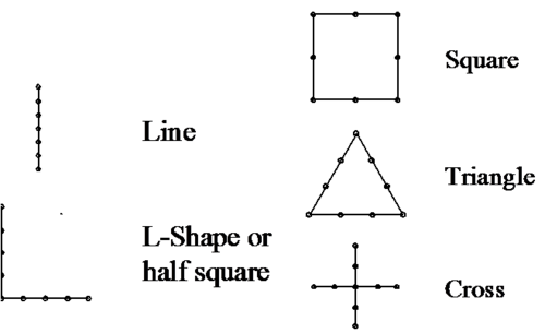
The above figure shows clusters with different geometric spatial arrangements of sub-plots. Each dot depicts one sub-plot. It is important to understand that the entire set of sub-plots is the observation unit or cluster (better: the cluster-plot). Sample size is determined by the number of clusters and not by the number of sub-plots.
 Info
Info
- This does often cause confusion but it is easy: we may call the entire cluster a cluster-plot; where the plot does not come in one compact piece (as with a circular fixed area plot) but is sub-divided into various distinct pieces. A cluster-plot can thus be viewed as a “funny shaped” plot.
It is a good terminology practice to always refer to “plot” if we talk about independently selected observation units. Therefore, the entire cluster is the plot (also called cluster-plot), and not the sub-plot. By erroneously referring to sub-plots as plots, one may cause confusion that may also lead to severe confusion about estimation as well.
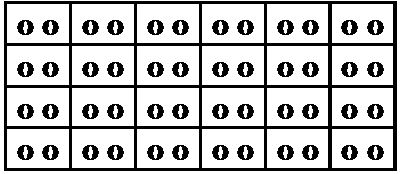
Coming back to an example, in the following figure the basic principle of cluster sampling is illustrated based on a population of 48 elements that is grouped into N=24 clusters of size m=2. In cluster sampling, this population of clusters constitutes the sampling frame from which sample elements are drawn. With each random selection a set of two individual elements is drawn which, however, does produce but one observation for estimation. That means the total or mean of the two elements (that is: an “aggregated” value) and not the two individual values is then further processed for estimation.
It has been mentioned that cluster plots, consisting of m sub-plots are standard in large area forest inventory, such as many National Forest Inventories.

Notation
As with stratified sampling, some notation needs to be introduced when developing the estimators for cluster sampling:
| \(N\,\) | Total population size = number of clusters in the population | |
| \(M\,\) | Numberof sub-plots in the population, \(M= \sum_{i=1}^N m_i\,\) | |
| \(\bar M\,\) | Mean cluster size in the population, \(\bar M=\frac{N}{M}\) | |
| \(n\,\) | Sample size = number of clusters in sample | |
| \(m_i\,\) | Number of sub-plots in cluster i, i.e. cluster size | |
| \(\bar m\,\) | Mean cluster size in the sample | |
| \(y_i\,\) | Observation in cluster i, i.e. total over all sub-plots of cluster i | |
| \(\bar y_i\) | Mean per sub-plot in cluster plot i = \(\bar y_i = \frac {y_i}{m_i}\) | |
| \(\bar y_c\,\) | Estimated mean per cluster in the sample = \(\bar y_c = \frac{1}{n} \sum_{i=1}^n y_i\) | |
| \(\bar y\,\) | Estimated mean per sub-plot in the sample = \(\bar y = \frac{1}{n} \sum_{i=1}^n \bar y_i\) |
Cluster sampling estimators
Clusters may have the same size \(m\) in terms of number of subplots for all clusters or variable size \(m_i\). Obviously, this needs to be taken into account in estimation. In this section, we present the estimator for the situation of cluster-plots of equal size under random sampling. When the population consists of clusters of unequal size, then the ratio estimator will likely yield more precise results, because the ratio estimator uses the cluster size as ancillary variable.
When all clusters have the same size, then \(m_i=\bar m\) is constant. The estimated mean per sub-plot can then be calculated from the estimated mean per cluster as:
\[\bar y = \frac{\bar y_c}{\bar m}\,\]
and the estimated error variance of the mean per sub-plot is:
\[\hat {var}_{cl} (\bar y) = \frac {1}{\bar m^2} \frac{N-n}{N} \frac{S_{y_i}^2}{n} \,\]
This reminds, obviously, to the error variance for simple random sampling, and only the first term is new\[S_{y_i}^2\] is the variance per cluster-plot; when we are interested in the variance per sub-plot, then the per-cluster variance needs to be divided by \(\bar m^2 \), similar to the estimated mean per sub-plot with the difference that \(\bar m\) is squared.
The estimated variance per cluster can be derived by calculating the variance over the per-cluster-observations:
\[S_{y_i}^2=\frac{\sum_{i=1}^n (y_i-\bar y_c)^2}{n-1}\]
The estimated total results as usual from multiplying the mean with the total; in cluster sampling, one may take the cluster mean and the number of clusters, or the mean per sub-plot and the number of sub-plots:
\[\hat \tau = N*\bar y_c = M * \bar y \,\],
where the error variance is
\[\hat {var} (\hat \tau) = N^2 \hat {var} (\bar y_c) = M^2 \hat {var} (\bar y) \,\].
The estimated error variance of the mean per sub-plot can alternatively be calculated from:
\[\hat {var}_{cl} (\bar y) = \frac {N-n}{N} \frac {1}{\bar m^2} \frac {\bar m^2 \sum_{i=1}^n (\bar y_i - \bar y)^2}{n-1} = \frac {N-n}{N} \frac {1}{n} \frac {\sum_{i=1}^n (\bar y_i - \bar y)^2}{n-1} \,\]
where \(S_{y_i}^2\) from the above error variance formula was replaced with \(S_{y_i}^2 = \bar m * S_{\bar y_i}^2\). It becomes obvious that this is exacly the simple random sampling estimator with the sub-plots as observation units and the variance of the sub-plots
\[S_{\bar y_i}^2 = \frac {\sum_{i=1}^n (\bar y_i - \bar y)^2}{n-1} \,\]
as estimated population variance. But remember that the sample size n is still the number of clusters, despite the fact that it is possible to use the sub-plot observations for estimation as well.
Cautions in cluster sampling
Unfortunately, an often committed error in cluster sampling is to treat the sub-plots as if they would be the independently selected sampling units. As a consequence the sample size appears to be much bigger than it actually is. And, because sample size n comes in the denominator of the error variance and the standard error estimator, this artificial inflation of sample size leads to a smaller value of the error variance. While, of course, smaller error variance is always welcome, in this case the smaller value comes from an erroneous calculation!
When interest is in producing point and interval estimates for the target variables, then an analysis of individual sub-plot observations is not help- nor useful. However, if interest is in assessing aspects of the spatial distribution of the variables of interest, then the sub-plot information may be of great interest because the cluster plot contains some information about the spatial relationships at defined distances.
 Cluster sampling examples: Examples for Cluster sampling
Comparison to SRS
If we compare cluster sampling to simple random sampling of the same number of sub-plots, then simple random sampling is expected to yield more precise results, because a much higher number of samples is being selected, covering more different situations of the population. While the cluster-plot, being a larger plot, will cover more variability within the plot, thus decreasing the variability between the plots; this smaller variance does usually not compensate the much smaller sample size.
 In simple words
- As in cluster sampling the observation from one cluster plot is derived as mean over all sub-plots, it can be assumed that more of the given variance can be captured inside a plot (or inside each single observation). The spatially dispersed sub-plots cover a wider range of conditions and by calculating the mean there is a compensating effect. Remember: The criterion for the quality of estimates is the standard error calculated based on the variance between the cluster plots (or observations). If more variance can be captured within the plots, the variance between the plots will decrease and the standard error will be lower (Means: an increase in precision).On the other hand, combining sub-plots to clusters leads to smaller sample size, as each cluster gives only one observation. Both effects can compensate each other.
However, the general statement of the preceding paragraph must be looked at in more detail: to what extent cluster sampling is statistically less efficient than simple random sampling depends exclusively on the covariance-structure of the population. This is dealt with in more detail in spatial autocorrelation and precision.
Cluster sampling is widely used in large area forest inventories, such as National Forest Inventories. The major reason does not lie in the statistical performance but in practical aspects: once a field team has reached a field plot location (which in some cases may take many hours or even some days), then one wishes to collect as much information as possible at this particular sample point. Therefore, it appears straightforward to establish a large plot and not a small one. Further on, large plots can be laid out in different manners: either as a compact individual plot – which, on the average, does not capture a lot of variability - or subdivided into sub-plots that are at a certain distance from each other – which tends to capture a lot more of variability. And, in addition, this spatial variability can also be analyzed.
References
- ↑ Kleinn, C. 2007. Lecture Notes for the Teaching Module Forest Inventory. Department of Forest Inventory and Remote Sensing. Faculty of Forest Science and Forest Ecology, Georg-August-Universität Göttingen. 164 S.
- ↑ Schindele, W. 1989. Field Manual for Reconnaissance Inventory on Burned Areas, Kalimantan Timur. FR-Report No.2.


