Cluster sampling examples
Example 1:
Assume that a study with relatively large square fixed area plots of 50 m x 50 m had been carried out, on which all tree positions were mapped. Because the individual plots were relatively large, there were only resources available to measure \(n=10\) sample plots. The small sample size led to a fairly high value of the estimated error variance.
A colleague of yours suggests: As you have mapped all trees on your 50 m x 50 m plot, you can easily make four plots of 25 m x 25 m out of each original plot. By that, you increase the sample size to the fourfold and, thus, reduce the error variance.
Does this suggestion seem reasonable?
Of course not!! The and the randomization scheme applied define what the independent observation unit is. In this case, each one of the 50 m x 50 m plots had been selected randomly and constitutes therefore one independent observation. This one single independent observation cannot be subdivided into more independent observations; it is just one. The sub-division may help learning about the spatial distribution of the variable of interest within the clusters and may, therefore, be very instructive for the optimization of the cluster plot design – but it does not help reducing the error variance (Kleinn 2007[1])!
Example 2:

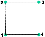
In a regional forest inventory in Northern Costa Rica, cluster plots of four sub-plots were used (as showed in figure 1), arranged at the corners of a square of 150 m side length. A sample of around 900 cluster plots was systematically laid out over the region of interest. At the center point of each sub-plot one may observe the dichotomous variable “forest-or-not” in order to produce an estimation of forest area.
At each one of the four sub-plots (points) the observation “1” (forest) or “0” (non-forest) is made so that for an entire cluster plot there are the following five possible values, depending how many sub-plots come to lie in forest: 0.0, 0.25, 0.5, 0.75 and 1.0. Table 1 gives summary statistics that are required for different approaches to area estimation and Table 2 gives the results for three approaches.
Table 1 Summary datas required for area estimation from cluster plots as of figure 1 (Kleinn 1993).
Data (inventory Zona Norte of Costa Rica)
(Kleinn 1993)Sample size of clusters \(n\) 899 Clusters with subplot no. 1 in forest 203 Clusters with forest subplots 282 Clusters with 1 forest subplot 52 Clusters with 2 forest subplot 60 Clusters with 3 forest subplot 58 Clusters with 4 forest subplot 114 Clusters without forest plots 617
- If the entire cluster-plots are (correctly) treated as observation units, the forest cover percent is estimated to \(22.3026%\) with a relative standard error of \(SE%=5.47%\).
- If we (incorrectly!!) treated the sub-plots as independent observations, then the forest cover estimate would be exactly the same, but the relative standard error would be much lower
\(SE%=2.81%\). However, as we know, this approach is wrong and we need to report the standard error that results from the correct cluster-plot analysis. - We may also ask whether (just for the purpose of area estimation) it was worthwhile to make four sub-observations per sample point or whether one single observation would maybe have been sufficient. Then, we can look at all cluster plots and analyze only the observation, for example, on sub-plot 1. The corresponding data are given in Table 1. This is a correct estimation in which we use only a part of the sample plot used (the cluster plot). The estimated forest cover is about the same \((22.5087%)\) and the standard error percent is slightly higher \(SE%=6.19%\); however, one may wonder whether the additional efforts of making 4 instead of 1 observation per sample point is really justified when the standard error can slightly be improved from \(6.19%\) to \(5.47%\)!
Table 2 Results for different approaches of area estimation. All clusters have the same size. Therefore, point estimation is the same whether entire clusters are analyzed or (incorrectly) the sub-plots.
Type of analysis Estimate Error Option I: entire clusters 0.223026 0.01220
5.47%Option II: only first cluster point 203/899=
0.2250870.013929
6.19%Incorrect
Treat all 4*899 subplots as
independent samples802/3596=
0.2230260.006259
2.81%
The fact that the precision of analyzing one sub-plot and analyzing four sub-plots is not very different is probably because of the relatively high intra-cluster correlation (see Spatial autocorrelation and precision). And this has likely to do with the geometric characteristics of forest fragmentation in the area of interest. The spatial extension of the cluster is obviously considerably smaller than the forest patches and the non-forest patches so that, if a sub-plot is in forest, the probability is high that other sub-plots lie also in forest; and even more so for non-forest as about 80% of the area is non-forest.
References
- ↑ Kleinn, C. 2007. Lecture Notes for the Teaching Module Forest Inventory. Department of Forest Inventory and Remote Sensing. Faculty of Forest Science and Forest Ecology, Georg-August-Universität Göttingen. 164 S.
- ↑ Kleinn C. 1993: Single tree volume estimation with multiple measurements using importance sampling and control variate sampling - an empirical study. IUFRO Conference on Modern Methods of Estimating Tree and Log Volume and Increment, June 14-16, 1993, Morgantown, West Virginia, USA.