Sampling with unequal selection probabilities
(→Importance sampling) |
(→Bitterlich sampling) |
||
| Line 176: | Line 176: | ||
| − | We saw, for example, that angle count sampling (Bitterlich sampling) selects the trees with a probability proportional to their [[basal area]] and we emphasized that this fact makes Bitterlich sampling so efficient for basal area estimation. In contrast, point to tree [[distance sampling]], or k-tree sampling, has inclusion zones that do not depend on any individual tree characteristic but only on the spatial arrangement of the neighboring trees; therefore, point-to tree distance sampling is not particularly precise for any tree characteristic. | + | We saw, for example, that angle count sampling ([[Bitterlich sampling]]) selects the trees with a probability proportional to their [[basal area]] and we emphasized that this fact makes [[Bitterlich sampling]] so efficient for basal area estimation. In contrast, point to tree [[distance sampling]], or k-tree sampling, has inclusion zones that do not depend on any individual tree characteristic but only on the spatial arrangement of the neighboring trees; therefore, point-to tree distance sampling is not particularly precise for any tree characteristic. |
| − | In Bitterlich sampling, the selection probability of a particular tree ''i'' results from the inclusion zone ''F<sub>i</sub>'' and the size of the reference area, for example the hectare | + | In [[Bitterlich sampling]], the selection probability of a particular tree ''i'' results from the inclusion zone ''F<sub>i</sub>'' and the size of the reference area, for example the hectare |
Revision as of 15:07, 12 January 2011
Contents |
Introduction
This article is, if not explicitly stated otherwise, based upon the lecturenotes for the teaching modul"Forest Inventory" by Kleinn et al. (2007[1]).
Mostly, one speaks about random sampling with equal selection probabilities: each element of the population has the same probability to be selected. However, there are situations in which this idea of equal selection probabilities does not appear reasonable: if it is known that some elements carry much more information about the target variable, they should also have a greater chance to be selected. Stratification goes into that direction: there, the selection probabilities within the strata were the same, but could be different between strata.
Sampling with unequal selection probabilities is still random sampling, but not simple random sampling, but “random sampling with unequal selection probabilities”. These selection probabilities, of course, must be defined for each and every element of the population before sampling and none of the population elements must have a selection probability of 0.
Various sampling strategies that are important for forest inventory base upon the principle of unequal selection probabilities, including
- angle count sampling (Bitterlich sampling),
After a general presentation of the statistical concept and estimators, these applications are addressed.
In unequal probability sampling, we distinguish two different probabilities – which actually are two different points of view on the sampling process:
The selection probability is the probability that element i is selected at one draw (selection step). The Hansen-Hurwitz estimator for sampling with replacement (that is; when the selection probabilities do not change after every draw) bases on this probability. The notation for selection probability is written as \(P_i\) or \(p_i\).
The inclusion probability refers to the probability that element i is eventually (or included) in the sample of size n. The Horvitz-Thompson estimator bases on the inclusion probability and is applicable to sampling with or without replacement. The inclusion probability is generally denoted by \(\pi\).
List sampling = PPS sampling
If sampling with unequal selection probabilities is indicated, the probabilities need to be determined for each element before sampling can start. If a size variable is available, the selection probabilities can be calculated proportional to size. This is then called PPS sampling (probability proportional to size).
Table 1. Listed sampling frame as used for „list sampling” where the selection probability is determined proportional to size.
Population element List of the size variables of the population elements List of cumulative sums Assigned range 1 10 10 0 - 10 2 20 30 > 10 - 30 3 30 60 > 30 - 60 4 60 120 > 60 - 120 5 100 220 > 120 - 220
This sampling approach is also called list sampling because the selection can most easily be explained by listing the size variables and select from the cumulative sum with uniformly distributed random numbers (which perfectly simulates the unequal probability selection process). This is illustrated in Table 1: the size variables of the 5 elements are listed (not necessarily any order!) and the cumulative sums calculated. The, uniformly distributed random number is drawn between the lowest and highest possible value of that range, that is from 0 to the total sum.
Assume, for example, the random number 111.11 is drawn; this falls into the range “>60 – 120” so that element 4 is selected. Obviously, the elements have then a selection probability proportional to the size variable.
Hansen-Hurwitz estimator
The Hansen-Hurwitz estimator gives the framework for all unequal probability sampling with replacement (Hansen and Hurwitz, 1943[2]). “With replacement” means that the selection probabilities are the same for all draws; if selected elements would not be replaced (put back to the population), the selection probabilities would change after each draw for the remaining elements.
Suppose that a sample of size n is drawn with replacement and that on each draw the probability of selecting the i-th unit of the population is \(p_i\).
Then the Hansen-Hurwitz estimator of the population total is
- \[\hat \tau = \frac {1}{n} \sum_{i=1}^n \frac {y_i}{p_i}\]
Here, each observation \(y_i\) is weighted by the inverse of its selection probability \(p_i\).
The parametric variance of the total is
- \[var (\hat \tau) = \frac {1}{n} \sum_{i=1}^N p_i \left (\frac {y_i}{p_i} - \tau \right )^2\]
which is unbiasedly estimated from a sample size n from
- \[v\hat ar (\hat \tau) = \frac {1}{n} \frac {\sum_{i=1}^n \left (\frac {y_i}{p_i} - \tau \right )^2}{n-1}\]
 Hansen-Hurwitz estimator examples: 4 application examples
Horvitz-Thompson estimator
Assuming that with any design, with or without replacement, the probability of including unit i in the sample is \(\pi_i\) (>0), for i=1,2,…, N. The inclusion probability \(\pi_i\) can be calculated from the selection probability \(p_i\) and the corresponding complementary probability (1-pi), which is the probability that the element is not included into the sample at a particular draw.
After n sample draws, the probability that element i is eventually included into the sample is \(\pi\)=1 - (1-pi)n, where (1 - pi)n is the probability that the particular element is not included after n draws; the complementary probability to this is then the probability that the element is eventually in the sample (at least selected once).
The Horvitz-Thompson estimator can be applied for sampling with or without replacement, but here it is illustrated for the case with replacement.
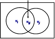
For the variance calculation with the Horvitz-Thompson estimator we also need to know the joint inclusion probability \(\pi_{ij}\) of two elements i and j after n sample draws, that is the probability that both i and j are eventually in the sample, after n draws. This joint inclusion probability is calculated from the two selection probabilities and the two inclusion probabilities after \(\pi_{ij} = \pi_i + \pi_j - \{ 1 - (1 - p_i - p_j)^n \} \) and can be illustrated as in Figure 1.
The Horvitz-Thompson estimator for the total is \(\hat \tau = \sum_{i=1}^\nu \frac {y_i}{\pi_i}\)
where the sum goes over the \(\nu\) distinc elements (where \(\nu\) is the Greek letter nu) in the sample of size n (and not over all n elements)
The parametric error variance of the total is
\[var(\hat \tau)=\sum_{i=1}^\nu \left (\frac {1 - \pi_i}{\pi_i} \right ) y_i^2 + \sum_{i=1}^N \sum_{j \ne i} \left (\frac {\pi_{ij} - \pi_i \pi_j}{\pi_i \pi_j} \right ) y_i y_j\]
which is estimated by
\[v\hat ar(\hat \tau)=\sum_{i=1}^\nu \left (\frac {1 - \pi_i}{\pi_i^2} \right ) y_i^2 + \sum_{i=1}^N \sum_{j \ne i} \left (\frac {\pi_{ij} - \pi_i \pi_j}{\pi_i \pi_j} \right ) \frac {y_i y_j}{\pi_{ij}}\]
A simpler (but slightly biased) approximation for the estimated error variance of the total is
\[v\hat ar(\hat \tau) = \frac {N - \nu}{N} \frac {1}{\nu} \frac {\sum_{i=1}^\nu (\tau_i -\hat \tau)^2}{\nu - 1}\]
where \(\tau_i\) is the estimation for the total that results from each of the \(\nu\) sample.
 Horvitz-Thompson estimator example: application example
Bitterlich sampling
For the inclusion zone approach where for each tree an inclusion zone is defined, see the corresponding article Infinite population approach. If used,the inclusion probability is then proportional to the size of this inclusion zone – which actually defines the probability that the correspondent tree is included in a sample.
We saw, for example, that angle count sampling (Bitterlich sampling) selects the trees with a probability proportional to their basal area and we emphasized that this fact makes Bitterlich sampling so efficient for basal area estimation. In contrast, point to tree distance sampling, or k-tree sampling, has inclusion zones that do not depend on any individual tree characteristic but only on the spatial arrangement of the neighboring trees; therefore, point-to tree distance sampling is not particularly precise for any tree characteristic.
In Bitterlich sampling, the selection probability of a particular tree i results from the inclusion zone Fi and the size of the reference area, for example the hectare
\[\pi_i = \frac {F_i}{10000}\]
with the Horvitz-Thompson estimator, we have the total
\[\hat \tau = \sum_{i=1}^m \frac {y_i}{\pi_i}\]
for any tree attribute \(y_i\). Applied to estimating basal area \(y_i = g_i = \frac {\pi}{4} d_i^2\) and its per hectare estimation, we have
\[\hat \tau = \sum_{i=1}^m \frac {y_i}{\pi_i} = \sum_{i=1}^m \cfrac {\cfrac {\pi}{4} d_i^2}{\cfrac {F_i}{10000}}\]
and with \( F_i = \pi r_i^2 = \pi c^2 \, d_i^2\), we have the same as Bitterlich
\[\hat \tau = \sum_{i=1}^m \frac {y_i}{\pi_i} = \sum_{i=1}^m \cfrac {\cfrac {\pi}{4} d_i^2}{\cfrac {\pi c^2 \, d_i^2}{10000}} = \frac {2500 \pi}{\pi c^2} \sum_{i=1}^m \frac {d_i^2}{d_i^2} = \frac {2500}{c^2} m\]
which is the estimated basal area per hectare from one sample point where m trees were tallied. The factor 2500/c² is the basal area factor, for details see Bitterlich.
Importance sampling
Importance sampling is a sampling strategy that selects samples proportional to size – but not from a discrete population of single elements of which each has a selection probability. Importance sampling is applicable to continuous populations where the size attribute is a function from which a probability density function is derived.
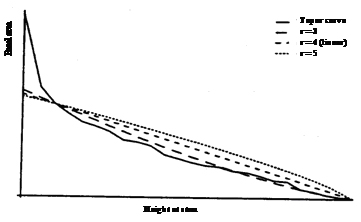
Typical application in forestry is estimating individual tree volume by sampling the taper curve: we imagine a taper curve is given, as for example, in Figure 2.
If A(h) is a function of basal area over height, the stem volume from the bottom to an upper height value \(H_u\) can be determined from
- \[\int_{0}^{H_u} A(h) dh\].
This integral is now to be estimated by selecting some heights at which basal area measurements are taken. One could select simple uniformly distributed height values and thus assigning the same selection probabilities to low height values where there is a lot of wood volume and the upper height values where there is much less volume. It makes, obviously, sense to use unequal selection probabilities that are continuously decreasing from the bottom to the top of the stem.
To do that, we must develop a scheme how to define the selection probabilities. In list sampling for discrete elements, we could craft a list and assign selection probabilities proportional to an ancillary size variable. With a continuous population we must devise a continuous function from which to sample with unequal probabilities. It would be optimal to know the exact taper curve, because then, we would make a perfect estimate of the target variable volume or area below the curve (just as we would make a perfect estimate of the totals with the Hansen-Hurwitz estimator if the selection probabilities can be defined strictly proportional to the target variable). As we do not know the taper curve, we use a proxy. Figure 2 shows various options together with the true taper curve of a sample tree. To build the proxy probability density function one needs input information; what we usually have is dbh and height, so that the proxy taper function goes through these points, where the curve intersects with the abscissa at tree height (tree radius = 0).
A probability density function (pdf) must have various properties:
- it must have positive values on the interval ;
- it must be 0 outside that interval;
- and the integral on the range \([H_b , H_u]\) must be 1.
All these conditions, by the way, are also satisfied when simple random sampling is applied. If the range of possible values is from 1…R, then the probability density function is a parallel to the abscissa intersecting the ordinate at the value 1/R; by that, it is guaranteed that the total probability density under the curve is 1.0.
A linear pdf is possible (r=4 in Figure 2). If is stem length (or total height), then the linear pdf takes on the form
- \[f(h) = \frac {2}{H_u} - \frac {2}{H_u^2} h \],
being defined on the range [0..\(H_u\)].
While the linear model works nicely in many cases, frequently a better approximation can be achieved by curves such as those of the form
- \[ d(h) = D \left [ \frac {H-h}{H} \right ]^{\frac {2}{r}}\]
Three examples for different values of the coefficient r are depicted in Figure 2.
If we select n sample heights \(\theta_i\) according to the pdf \(f(\theta_i)\) and measure there basal area \(A(\theta_i)\), then the volume V of that particular tree is estimated by the Hansen-Hurwitz estimator
- \[V = \frac {1}{n} \sum_{i=1}^n \frac {a(\theta_i}{f(\theta_i)}\].
We denote with \(V_p\) the volume that results from the proxy function \(A_p (h)\) on the interval from 0 to Hu. It is a biased volume as \(A_p (h)\) is but a proxy for the true function of basal area over height. The probability density function f(h) is then for
- \[0 \le h \le H_u \, f(h) = \frac {A_p (h)}{V_p}\]
Then, the volume estimation from measurements at n Heights at the stem - selected according to the pdf f(h) - can be re-written as
- \[\hat V = V_p \frac {1}{n}\sum_{i=1}^n \frac {A(\theta_i)}{A_p(\theta_i)}\],
where the expression to the right can be interpreted as a "calibration factor" which makes the estimation Vp unbiased.
The parametric error variance of volume estimation from a sample of size n is
- \[var(\hat V) = \frac {1}{n} \int_{H_U}^{H_O} f(h) \left [ \frac {A(h)}{f(h)} - V \right ]^2 dh = \frac {1}{n} \int_{H_U}^{H_O} \frac {A^2(h)}{f(h)} dh - V\,\] esttimated from a sample of size n from
- \[v\hat ar(\hat V) = \frac {1}{n(n-1)} \sum_{i=1}^n \left [ \frac {A(\theta_i)}{f(\theta_i)} - \hat V \right ]^2\].
For illustration: for a sampling study, the taper curve of various trees was accurately determined by many measurements. Then, it is possible to simulate different sampling approaches for the estimation of stem volume (Kleinn 1993 [3]). This was done for several hundred sample trees (spruce and Douglas fir). Then, the performance of different proxy functions (which define the unequal selection probabilities) was compared. The results are presented in Table 25. With simple random sampling the per-tree volume estimation with n = 1 has here a relative standard error of about 70% - which can, of course, only be determined by simulation, as a single sample of n = 1 does not allow estimating error variance. A linear probability density function (defined by tree height and the default measurement at breast height) yields a reduction of the relative standard error down to about 17%, which can still be improved by using a curvilinear probability density function (r=3 along the function given above; see also Table 2).
Table 2. Result from a simulation study on several hundred of trees (spruce and Douglas fir). Given is the mean relative error (cv%) of the volume estimate for importance sampling of individual trees with one measurement per tree (n=1) (from Kleinn 1993[3]). The estimations are given for different approaches to unequal probability sampling where the function \(d(h) = D \left [ \frac {H-h}{H} \right ]^{\frac {2}{r}}\) was used to define the shape of the proxy probability function. “Uniform” means simple random sampling from a uniform distribution of random numbers.
Species Uniform Linear pdf Pdf from proxy fuction with r=3 r=5 Norway spruce 69.8 17.8 12.9 25.0 Douglas fir 70.2 16.2 9.8 24.5
Randomized branch sampling
Total tree bark volume is a variable that cannot easily be directly measured. The “true” volume could theoretically be determined by stripping off all bark and using water displacement to measure volume. However, this is impractical and the obvious way to go is to develop simple models based on pragmatic sampling techniques.
To sample variables such as bark we imagine the tree as a population of above ground N stem and branch sections where each section goes from one fork (or node) to the next – except for the bottom and top sections at which the tree begins and ends, respectively. From this set of N sections we would then select n sections as sample.
Doing so by simple random sampling (SRS), for example, we could directly estimate the mean bark volume per section. However, for estimation of the total, we would then face the problem that we needed to know the population size, i.e. the total number of sections to determine the expansion factor to extrapolate the mean section estimate to the whole tree. If the population size is known, we also know the selection probability for each section ‑ 1/N for simple random sampling ‑: this selection probability is required to develop an unbiased estimator for any design based sampling strategy. This is what we call probabilistic sampling.
In addition, to be able to carry out simple random selection, we also need to define the sampling frame so that we can unambiguously identify individual sampling elements (sections, in our case). Both tasks (finding the population size and then defining the sampling frame), are clearly impractical for estimating total tree bark utilizing a simple random sampling approach.
Randomized branch sampling (RBS) is a sampling strategy that facilitates the drawing of a probabilistic sample without a priori defining the sampling frame. The selection probabilities of the selected population elements are determined in the course of the sampling process itself. RBS was developed by Jessen (1955)[4] for estimation of fruit count in orchards and has since been successfully applied to estimation of various tree variables (e.g. Valentine et al. 1984[5], Gregoire et al. 1995[6], Good et al. 2001[7], Cancino 2003, Cancino and Saborowski 2005[8]).
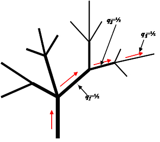
The principle of RBS can be visualized as a randomized unidirectional walk on a path along the network of stem sections starting from the bottom of the tree or another defined starting point to a defined end point (in our case up to a minimum branch diameter of 5 cm). Going along the path, at each fork a probability-based decision (utilizing random number tables or dice) is made to select the branch along which to proceed. Therefore, for each fork, the selection probability qi for the next section i is known. This permits the calculation of the overall selection probability for each section within the path as the product of the selection probabilities of all preceding sections. In Figure 3, for illustration, the marked outmost section has selection probability \(p_3 = q_1 * q_2 * q_3\). In that case, the first section (the stem) has selection probability \(q_0 =1\) and therefore also \(p_0 = 1\) because that section is part of all possible sample paths.

Knowing the selection probability for each section of a path, an estimator for the total of the target variable can be developed using the Hansen-Hurwitz estimator. The total \(\tau\) can then be estimated from one path of m sections \(y_i\) selected with probabilities \(p_i\) by
- \[ \hat \tau = \frac {1}{m} \sum_{i=1}^m \frac {y_i}{p_i}\].
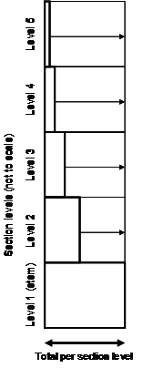
| Figure 4. Illustration of estimation in randomized branch sampling (after Good et al. 2001[7]): for each section level, the observed value (bold rectangle) is expanded to an estimated total value by dividing that value by its selection probability which is indicated here by the arrows. The sum of all expanded values is the estimation of the tree´s total. The stem has selection probability 1 so that no expansion takes place. Obs: The heights of the sections are set equal here while, of course, they vary within and between sections. The width of the section levels is set to 100% here; the absolute values would also vary. | 
|
Following statistical sampling principles one path provides one independent observation. This observation is composed of several “sub‑observations”, the sections. This is the same principle which is also applied in relascope sampling, where from one sample point various sample trees are included with selection probabilities proportional to their basal area; the sample tree values are then combined to one sample point observation by weighting them according to their individual selection probabilities. For randomized branch sampling the estimation mechanism is illustrated in Figure 4: dividing the observed section value by its per-section selection probability provides an estimation of the total on this section level (Good et al. 2001[7]).
If one path constitutes a sample of size n = 1, then more paths need to be selected per tree if estimation of precision is an issue. From n selected paths we generate n bark volume estimations \( \hat V_j\) the mean of which is taken as best estimate
- \[\bar V = \frac {1}{n} \sum_{j=1}^n \hat V_j \]
with estimated variance
- \[v\hat ar (\bar V) = \frac {s^2}{n} = \frac {1}{n} \frac {\sum_{j=1}^n (\hat V_j - \bar V)^2}{(n-1)}\].
References
- ↑ Kleinn, C.2007. Lecture Notes for the Teaching Module ForestInventory. Departmentof Forest Inventory and Remote Sensing. Facultyof Forest Science andForest Ecology, Georg-August-UniversitätGöttingen. 164 S.
- ↑ Hansen MM and WN Hurwitz. 1943. On the theory of sampling from finite populations. Annals of Mathematical Statistics 14:333-362.
- ↑ 3.0 3.1 Kleinn C. 1993: Single tree volumeestimation with multiple measurements using importance sampling andcontrol variate sampling - an empirical study. IUFRO Conference onModern Methods of Estimating Tree And Log Volume and Increment, June14-16, 1993, Morgantown, West Virginia, USA.
- ↑ Jessen R.J. 1955. Determining the fruit count on a tree by randomized branch sampling. Biometrics 11:99-109
- ↑ Valentine TV, LM Tritton and GM Furnival. 1984. Subsampling Trees for Biomass, Volume or Mineral Content. Forest Science 30(3):673-681
- ↑ Gregoire TG, HT Valentine and GM Furnival. 1995. Sampling methods to estimate foliage and other characteristics of individual trees. Ecology 76:1181-1194
- ↑ 7.0 7.1 7.2 Good NM, M Paterson, C Brack and .K Mengersen. 2001. Estimating Tree Component Biomass Using Variable Probability Sampling Methods. Journal of Agricultural, Biological, and Environmental Statistics 6(2):258–267
- ↑ Cancino J and J Saborowski. 2005. Comparison of randomized branch sampling with and without replacement at the first stage. Silva Fennica 39(2):201-216.

