Inclusion probability

[−] Forest inventory

[+] Introduction to forest inventory

[+] Forest mensuration

[+] Introduction to sampling

[+] Plot design

[+] Sampling design

[+] Estimation issues

[+] Planning issues

[+] UNFCCC Implications for Forest Monitoring

[+] Forest Inventory Examples

  Forest Inventory Glossary

In probabilistic sampling each element of the population must have a non-zero probability to be included in a sample, otherwise unbiased estimation is not possible. The reason therefore is very simple: If not all elements of a population have a positive probability to become part of a sample, one can not expect that an actual sample is able to describe the unknown population parameters correctly. The inclusion probability \({\pi}_i\,\) refers to the chance that the \(i^{th}\) population element becomes part of a sample. The inclusion probability should be distinguished from the selection probability \(p(s)\) of a sample that is the probability that a certain unordered set of elements (e.g. a number of trees included by a sample plot) is selected as sample.

Inclusion zone concept

Sampling for forest attributes is in some aspects not directly comparable to basic statistical concepts we often learn in school. Contrary to basic examples of probabilistic sampling, like the probabilities in a deck of cards or other finite populations, sampling for area related forest attributes take place in an infinite areal sampling frame. As the random selection of samples is based on the selection of dimensionless points in an area of interest, there is an infinite number of possibilities.

Important!

Please always remember that the population we take samples of, is not the biological population of trees. Sampling in forestry is based on the selection of sample points and not trees. Afterwards an observation is derived by including trees at which we take the measurements (normally this is not only one tree, but e.g. all trees on a plot). Nevertheless we need to know the inclusion probability of each tree to derive an unbiased estimate for the target variable. This probability is the inverse of the expansion factor that one has to apply if an estimate of the total is targeted.

To determine the inclusion probability of a single tree, one has to know the relative share of all possible sample point locations that would lead to its inclusion, related to the total area of interest (or one hectare if the values should be reported to this reference). This locus of points is also known as inclusion zone. As the number of points is infinite, the area of this region is used as measure for the probability. 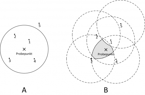With the below figure this concept is explained for fixed area plots. On the left side (A) a sample plot is installed around a selected sample point (cross). Obviously tree 1, 2, 3 and 4 are inside the plot (included). In the right figure (B) the inclusion zones are delineated for all trees (dashed line). In case of fixed area plots they are of same shape and size as the sample plot, but centered at the tree location. In case of unequal probability sampling (like e.g. Bitterlich sampling or a nested plot design), tree individual inclusion zones might be of various size. For each of these trees, a sample point falling in its inclusion zone, would lead to an inclusion of the respective tree.

The gray shaded area in figure B is expression of the selection probability of this special set of trees (all sample points falling inside this area would lead to an inclusion of the same set of trees, and consequently select the same sample). It is obvious that this probability is unknown and can hardly be determined in the field. Nevertheless it's intuitively clear, that a randomly placed sample point will select a certain sample with a probability proportional to the size of this area.

Note

In case that the locations of all objects in an area of interest are known (e.g. in case that data of tree positions for a larger experimental plot are available), it is possible to compute a tessellation of the areal sampling frame in mutually exclusive polygons, each related to a certain observation at this locus of points. This approach is very suitable if the performance of different plot designs should be compared, as all statistical aspects of the respective design can be derived analytically. This approach is also known as the jigsaw puzzle view (Roesch et al. 1993).

References

- ↑ Roesch, F.A.; Green,E.J.; Scott, C.T. 1993. An Alternative View of Forest Sampling. Survey Methodology 19 (2), 199-204.