GSG
(→GSG application) |
|||
| (22 intermediate revisions by one user not shown) | |||
| Line 19: | Line 19: | ||
===GSG application=== | ===GSG application=== | ||
Given a unified framework to generate sampling grids, the question remains how to make use of this for a sample based estimation of specific target variables? The GSG generates dimensionless sampling locations (points), but how to come to meaningful observations as basis for statistical estimations? A central aspect of the GSG project is to answer this question, depending on different target variables. Contrary to the most common approach of creating model-based wall-to-wall predictions from remote sensing imagery, we are focusing on visual interpretation of relatively small samples. These could be obtained by classifying the dimensionless sampling locations according to a suitable land-cover/land-use classification key that needs to be developed under consideration of the actual image resolution. A simple example would be the estimation of forest cover by the GSG points as observation units (see [[Estimating forest area]]). | Given a unified framework to generate sampling grids, the question remains how to make use of this for a sample based estimation of specific target variables? The GSG generates dimensionless sampling locations (points), but how to come to meaningful observations as basis for statistical estimations? A central aspect of the GSG project is to answer this question, depending on different target variables. Contrary to the most common approach of creating model-based wall-to-wall predictions from remote sensing imagery, we are focusing on visual interpretation of relatively small samples. These could be obtained by classifying the dimensionless sampling locations according to a suitable land-cover/land-use classification key that needs to be developed under consideration of the actual image resolution. A simple example would be the estimation of forest cover by the GSG points as observation units (see [[Estimating forest area]]). | ||
| − | As preliminary work to the project we implemented a small sampling study based on a time series of Landsat lookup images of the district Buritis in Northern Randônia, Brazil. The classification of points from a GSG with 10km resolution into forest or non-forest is basis to estimate forest cover and its changes over time. The respective GSG_10 subset and the imagery used can be found on the [http://134.76.21.147/maps/382 AWF-Geoserver] (open map and zoom to Brazil). The following figure shows some of the available | + | As preliminary work to the project we implemented a small sampling study based on a time series of Landsat lookup images of the district Buritis in Northern Randônia, Brazil. The classification of points from a GSG with 10km resolution into forest or non-forest is basis to estimate forest cover and its changes over time. The respective GSG_10 subset and the imagery used can be found on the [http://134.76.21.147/maps/382 AWF-Geoserver] (open map and zoom to Brazil). The following figure shows some of the available acquisitions: |
[[File:Randonia.png|center]] | [[File:Randonia.png|center]] | ||
| + | [[File:line.png|thumb|350px|[[line sampling]]]] | ||
| + | [[File:point_cluster.png|thumb|350px|[[cluster sampling]] with point grid]] | ||
| + | [[File:fixed_area_plot.png|thumb|350px|2-dimesnional sample plot]] | ||
An estimate of forest cover change and its standard error over time leads to the following result (Error bars represent the absolute standard error of the estimated cover percentage): | An estimate of forest cover change and its standard error over time leads to the following result (Error bars represent the absolute standard error of the estimated cover percentage): | ||
[[File:Randonia_results.png|center]] | [[File:Randonia_results.png|center]] | ||
| + | |||
| + | It is obvious that the precision of forest cover estimates is decreasing with decreasing forest cover in this example. This is because forest becomes a rare event over time. Sampling for rare events is a science in itself and there are whole textbooks about that specific topic. Often, the simplest solution is to increase sample size in order to increase the probability to encounter the rare objects; however, this increases labor cost as well. Another option to increase the [[inclusion probability]] of remaining forest patches is to adapt the observation design. Sometimes also techniques like [[adaptive cluster sampling]] are applied to rare classes. | ||
===Optimazation of observation units=== | ===Optimazation of observation units=== | ||
| − | For many applications it might be statistically much more efficient to define a suitable [[:category:plot design|observation design]] that is attached to each sampling location. In statistical sampling the [[Accuracy and precision|precision]] of estimates can be influenced in different ways. The sampling design, especially the [[sample size]], has a strong influence on the resulting precision of estimates that is quantified by the [[standard error]]. However, also the design of the observation units that are implemented at each sample point affects the precision of estimates. As a general guideline, and contrary to the design planning of experimental plots, the observation units in an observational design (inventory type) should be designed such that each observation unit is as heterogeneous as possible, | + | For many applications it might be statistically much more efficient to define a suitable [[:category:plot design|observation design]] that is attached to each sampling location. In statistical sampling the [[Accuracy and precision|precision]] of estimates can be influenced in different ways. The sampling design, especially the [[sample size]], has a strong influence on the resulting precision of estimates that is quantified by the [[standard error]]. However, also the design of the observation units that are implemented at each sample point affects the precision of estimates. As a general guideline, and contrary to the design planning of experimental plots, the observation units in an observational design (inventory type) should be designed such that each observation unit is as heterogeneous as possible, thus capturing as much as possible of the variability of a target variable; this feature does eventually reduce the error variance between the observation (viz. increases precision). |
| − | The options to define the units on which observations are made are manifold. It might be a cluster of points, which are secondary sampling units in this case (see [[cluster sampling]]), line elements (see [[Line sampling]]) or 2-dimensional sample plots. In any case the statistical estimation design is a consequence of the applied observation design. Unbiased estimation of target variables is only possible if the applied observation protocol is considered correctly. | + | The options to define the units on which observations are made are manifold. It might be a cluster of points, which are secondary sampling units in this case (see [[cluster sampling]]), line elements (see [[Line sampling]]) or 2-dimensional sample plots. In the right figures examples of these alternatives are overlaid over the same image subset. Of course there are many more options and a methodological approach how to design the observation units such that the overall efficiency (dependent on resulting precision and classification effort) is possibly high, would be very helpful. In any case the statistical estimation design is a consequence of the applied observation design. Unbiased estimation of target variables is only possible if the applied observation protocol is considered correctly. |
| − | Besides the general concept of observation units they can be adapted to special circumstances in terms of size and configuration. In this context an analysis of within-plot [[Spatial autocorrelation]] can give insights into their statistical efficiency. | + | Besides the general concept of observation units they can be adapted to special circumstances in terms of size and configuration. In this context an analysis of within-plot [[Spatial autocorrelation]] can give insights into their statistical efficiency. |
| − | + | Looking to the figures on the right it is obvious that the observation of the target variable (here its about forest cover. yellow = forest, blue = non-forest) is related to different "observation efforts". Mapping the land cover on the 2-dimensional plot area takes much longer than classifying the points or line segments. The evaluation of statistical performance of different alternatives is part of the research program of the GSG project. | |
| − | + | ||
| − | + | ||
| − | + | ||
| − | + | ||
===GSG R code=== | ===GSG R code=== | ||
| + | A short example of the R-code used to generate GSGs is given below. Eventually you need to install the required packages first (by uncommenting and running the first 4 lines). | ||
| + | If you run this example it should result in a GSG_100 for Canada (you need to specify your output location before exporting the grid to a .kml file). It is important to note that each individual grid that is generated is part of the overall global grid system (and not an independent local grid). | ||
| + | [[File:GSG_100_CAN.jpg|thumb|350px|Google Earth screen shot of the GSG_100 for Canada as produced with the given R-code.]] | ||
<source lang="rsplus"> | <source lang="rsplus"> | ||
############################################################################# | ############################################################################# | ||
| Line 45: | Line 49: | ||
############################################################################# | ############################################################################# | ||
#by Lutz Fehrmann | #by Lutz Fehrmann | ||
| + | |||
| + | # install.packages("sp") # Instalation of the required packages | ||
| + | # install.packages("rgdal") # Instalation of the required packages | ||
| + | # install.packages("maptools") # Instalation of the required packages | ||
| + | # install.packages("rgeos") # Instalation of the required packages | ||
# Specify your output location and file name for kml export | # Specify your output location and file name for kml export | ||
| Line 50: | Line 59: | ||
file.name <- "test" # e.g. specification of the aoi | file.name <- "test" # e.g. specification of the aoi | ||
| − | # Set distance between points in km | + | # Set distance between points along latitudes in km |
d = 100 | d = 100 | ||
| Line 57: | Line 66: | ||
# To compute a global grid use default c(-90, 90, -180, 180) | # To compute a global grid use default c(-90, 90, -180, 180) | ||
aoi <- c(-90, 90, -180, 180) | aoi <- c(-90, 90, -180, 180) | ||
| − | |||
# Optional: Compute grid for a specific country: Enter ISO3 country code | # Optional: Compute grid for a specific country: Enter ISO3 country code | ||
| Line 93: | Line 101: | ||
# Subset gridpoints falling on land (or in a specific country) | # Subset gridpoints falling on land (or in a specific country) | ||
| − | |||
library("rgeos") | library("rgeos") | ||
| + | library("maptools") | ||
# load country polygons (from package maptools) | # load country polygons (from package maptools) | ||
| Line 109: | Line 117: | ||
# Plot preview map of aoi ------------ | # Plot preview map of aoi ------------ | ||
| − | |||
| − | |||
plot(wrld_trans[wrld_trans$ISO3==country,], col = gray(.95), axes = T) | plot(wrld_trans[wrld_trans$ISO3==country,], col = gray(.95), axes = T) | ||
points(GSGcountry, pch = 20, cex = 0.1, col = "red") | points(GSGcountry, pch = 20, cex = 0.1, col = "red") | ||
| Line 116: | Line 122: | ||
# Optional: Output of grid coordinates as .kml file for Google Earth or GIS | # Optional: Output of grid coordinates as .kml file for Google Earth or GIS | ||
# Export kml file of the whole global grid with specified point distance ------------- | # Export kml file of the whole global grid with specified point distance ------------- | ||
| − | # writeOGR(GSGsp, paste(output.location, "GSG", d, "_global_", file.name, ".kml", sep = ""), layer = paste("GSG_", d, "_kml", sep = ""), driver = "KML") | + | # writeOGR(GSGsp, paste(output.location, "GSG", d, "_global_", file.name, ".kml", sep = ""), |
| + | # layer = paste("GSG_", d, "_kml", sep = ""), driver = "KML") | ||
# Export .kml file of the subset of gridpoints on land ------------ | # Export .kml file of the subset of gridpoints on land ------------ | ||
| − | # writeOGR(GSGland, paste(output.location, "GSG", d, "_land_", file.name, ".kml", sep = ""), layer = paste("GSG_", d, "_kml", sep = ""), driver = "KML") | + | # writeOGR(GSGland, paste(output.location, "GSG", d, "_land_", file.name, ".kml", sep = ""), |
| + | # layer = paste("GSG_", d, "_kml", sep = ""), driver = "KML") | ||
# Export .kml file of gridpoints for selected country only ---------- | # Export .kml file of gridpoints for selected country only ---------- | ||
| − | writeOGR(GSGcountry, paste(output.location, "GSG", d, "_", country, "_", file.name, ".kml", sep = ""), layer = paste("GSG_", d, "_kml", sep = ""), driver = "KML") | + | writeOGR(GSGcountry, paste(output.location, "GSG", d, "_", country, "_", file.name, ".kml", sep = ""), |
| + | layer = paste("GSG_", d, "_kml", sep = ""), driver = "KML") | ||
</source> | </source> | ||
Latest revision as of 08:29, 15 December 2016
Contents |
[edit] A unified framework for environmental monitoring based on a discrete global sampling grid system (GSG)
[edit] Background
Environmental monitoring on different spatial scales is a key element in many international and national processes related to ecological and environmental challenges. The increasing availability of large archives of freely available high resolution and Geo-referenced imagery through virtual globes like Google Earth, Microsoft Virtual Earth (bing) or NASA World Wind and others is still relatively underexploited by scientific applications in this context. Even if these information sources are frequently used by scientists, e.g. for communication and visualization of project activities or even as basis for observations in remote sensing imagery, there is hardly any methodological framework that helps to make use of the data sources for sample based estimation. Depending on the available spatial resolution of images, many relevant target variables, like e.g. forest cover, could be interpreted visually and could serve as basis for statistical estimation on larger areas.
[edit] Concept of a discrete global sampling grid
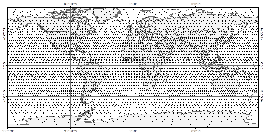
We propose a very simple and easy to communicate discrete global grid system (Global Sampling Grid = GSG) that could serve as basic sampling design from global to local scale. The grid construction follows a simple approach: Circles of latitudes are placed with a constant distance on the surface of a sphere with radius of 6378.137 m (major axis of the World Geodetic System, WGS84) outgoing from the equator in North and South direction. On each of these latitudes sampling locations are placed in the same constant distance outgoing from the Greenwich meridian in West and East direction. This leads to a half systematic arrangement of sampling locations, where the distance of points is constant along the latitudes. Here a global GSG with a point distance of 250km is shown in a cylindrical map projection.
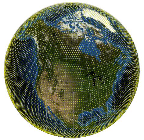
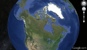
The half-systematic design of this grid might become more obvious if draped over a spherical projection of the earth surface, like e.g. used by virtual globes. If exported to a .kml file and shown in Google Earth a GSG with 100km point distance (GSG_100_global) looks like this:
Other examples of GSG subsets can be found on the AWF-Geoserver of the Chair of Forest Inventory and Remote Sensing at the Georg-August-Universität Göttingen. An R package to create grids in any scale and any region of the world has been developed. All grids have the same origin and sampling locations from affine grids of different resolution coincide. This makes the GSG very interesting if data from different sampling studies should be compiled; this is of particular interest for example, for international environmental policy processes and their monitoring instruments, and for internationally acting organizations. A lot of synergies and option for analyzing data are arising if environmental monitoring and sampling studies from other disciplines are combined. One objective of the GSG project is to further develop a R package that allows to construct grids in different spatial resolution and for different regions that are all part of the overall grid system. As preliminary work to the project we developed a basic GSG R code that will be further extended.
[edit] GSG application
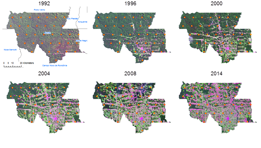
Given a unified framework to generate sampling grids, the question remains how to make use of this for a sample based estimation of specific target variables? The GSG generates dimensionless sampling locations (points), but how to come to meaningful observations as basis for statistical estimations? A central aspect of the GSG project is to answer this question, depending on different target variables. Contrary to the most common approach of creating model-based wall-to-wall predictions from remote sensing imagery, we are focusing on visual interpretation of relatively small samples. These could be obtained by classifying the dimensionless sampling locations according to a suitable land-cover/land-use classification key that needs to be developed under consideration of the actual image resolution. A simple example would be the estimation of forest cover by the GSG points as observation units (see Estimating forest area). As preliminary work to the project we implemented a small sampling study based on a time series of Landsat lookup images of the district Buritis in Northern Randônia, Brazil. The classification of points from a GSG with 10km resolution into forest or non-forest is basis to estimate forest cover and its changes over time. The respective GSG_10 subset and the imagery used can be found on the AWF-Geoserver (open map and zoom to Brazil). The following figure shows some of the available acquisitions:
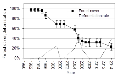
An estimate of forest cover change and its standard error over time leads to the following result (Error bars represent the absolute standard error of the estimated cover percentage):
It is obvious that the precision of forest cover estimates is decreasing with decreasing forest cover in this example. This is because forest becomes a rare event over time. Sampling for rare events is a science in itself and there are whole textbooks about that specific topic. Often, the simplest solution is to increase sample size in order to increase the probability to encounter the rare objects; however, this increases labor cost as well. Another option to increase the inclusion probability of remaining forest patches is to adapt the observation design. Sometimes also techniques like adaptive cluster sampling are applied to rare classes.
[edit] Optimazation of observation units
For many applications it might be statistically much more efficient to define a suitable observation design that is attached to each sampling location. In statistical sampling the precision of estimates can be influenced in different ways. The sampling design, especially the sample size, has a strong influence on the resulting precision of estimates that is quantified by the standard error. However, also the design of the observation units that are implemented at each sample point affects the precision of estimates. As a general guideline, and contrary to the design planning of experimental plots, the observation units in an observational design (inventory type) should be designed such that each observation unit is as heterogeneous as possible, thus capturing as much as possible of the variability of a target variable; this feature does eventually reduce the error variance between the observation (viz. increases precision).
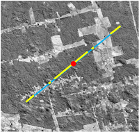
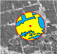
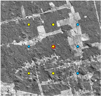
The options to define the units on which observations are made are manifold. It might be a cluster of points, which are secondary sampling units in this case (see cluster sampling), line elements (see Line sampling) or 2-dimensional sample plots. In the right figures examples of these alternatives are overlaid over the same image subset. Of course there are many more options and a methodological approach how to design the observation units such that the overall efficiency (dependent on resulting precision and classification effort) is possibly high, would be very helpful. In any case the statistical estimation design is a consequence of the applied observation design. Unbiased estimation of target variables is only possible if the applied observation protocol is considered correctly. Besides the general concept of observation units they can be adapted to special circumstances in terms of size and configuration. In this context an analysis of within-plot Spatial autocorrelation can give insights into their statistical efficiency.
Looking to the figures on the right it is obvious that the observation of the target variable (here its about forest cover. yellow = forest, blue = non-forest) is related to different "observation efforts". Mapping the land cover on the 2-dimensional plot area takes much longer than classifying the points or line segments. The evaluation of statistical performance of different alternatives is part of the research program of the GSG project.
[edit] GSG R code
A short example of the R-code used to generate GSGs is given below. Eventually you need to install the required packages first (by uncommenting and running the first 4 lines).
If you run this example it should result in a GSG_100 for Canada (you need to specify your output location before exporting the grid to a .kml file). It is important to note that each individual grid that is generated is part of the overall global grid system (and not an independent local grid).
#############################################################################
#                            GLOBAL SAMPLING GRID  (GSG)                    #
#############################################################################
#by Lutz Fehrmann

# install.packages("sp")       # Instalation of the required packages
# install.packages("rgdal")    # Instalation of the required packages
# install.packages("maptools") # Instalation of the required packages
# install.packages("rgeos")    # Instalation of the required packages

# Specify your output location and file name for kml export
output.location <- "D:/Projects/GSG/GSG_export/"
file.name <- "test" # e.g. specification of the aoi

# Set distance between points along latitudes in km
d = 100

# Optional: Define area of interest (aoi) in a rectangular envelope
# c(min Lat, max Lat, min Lon, max Lon) in decimal degree!
# To compute a global grid use default c(-90, 90, -180, 180)
aoi <- c(-90, 90, -180, 180)

# Optional: Compute grid for a specific country: Enter ISO3 country code
# (http://en.wikipedia.org/wiki/ISO_3166-1_alpha-3#Current_codes)
country <- "CAN"

# Calculate grid coordinates ------------
# The grid is systematic (equidistant points along cicles of latitude)
# on a spheroid (WGS84/Pseudo-Mercator, epsg:3857)
# Calculate the angle of an d-arc in degree
deg <- (d/(pi * 6378.137)) * 180

# Create a vector of longitue along equator
longitude <- sort(c(seq(0, -180, -deg), seq(deg, 180, deg)))

# Create a vector of latitudes in aoi
latitudes <- longitude[longitude >= aoi[1] & longitude <= aoi[2]]

# Calculate a matrix of longitudes for each circle of latitude
longitudes <- outer(longitude, latitudes, function(x,y) x/cos(pi/180 * y))

# Compile coordinates
coordinates<-cbind(as.vector(t(longitudes)), latitudes)
colnames(coordinates)<-c("X","Y")

# Subset coordinates in aoi
coordinates<-coordinates[coordinates[,1] >= aoi[3] & coordinates[,1] <= aoi[4],]

# To SpatialPointDataFrame
library("rgdal")
GSGsp <- SpatialPointsDataFrame(cbind(coordinates[,1], coordinates[,2]),
                                data = data.frame(1:nrow(coordinates)))
# Assign projection (longlat +datum=WGS84)
proj4string(GSGsp) <- CRS("+init=epsg:4326")

# Subset gridpoints falling on land (or in a specific country)
library("rgeos")
library("maptools")

# load country polygons (from package maptools)
data(wrld_simpl)

# Set projection
wrld_trans <- spTransform(wrld_simpl, CRS("+init=epsg:4326"))

# Subset points on land
GSGland <- GSGsp[wrld_trans,]

#subset per country
GSGcountry <- GSGland[wrld_trans[wrld_trans$ISO3==country,],]

# Plot preview map of aoi ------------
plot(wrld_trans[wrld_trans$ISO3==country,], col = gray(.95), axes = T)
points(GSGcountry, pch = 20, cex = 0.1, col = "red")

# Optional: Output of grid coordinates as .kml file for Google Earth or GIS
# Export kml file of the whole global grid with specified point distance -------------
# writeOGR(GSGsp, paste(output.location, "GSG", d, "_global_", file.name, ".kml", sep = ""),
# layer = paste("GSG_", d, "_kml", sep = ""), driver = "KML")

# Export .kml file of the subset of gridpoints on land ------------
# writeOGR(GSGland, paste(output.location, "GSG", d, "_land_", file.name, ".kml", sep = ""),
# layer = paste("GSG_", d, "_kml", sep = ""), driver = "KML")

# Export .kml file of gridpoints for selected country only ----------
writeOGR(GSGcountry, paste(output.location, "GSG", d, "_", country, "_", file.name, ".kml", sep = ""),
layer = paste("GSG_", d, "_kml", sep = ""), driver = "KML")
