Spatial autocorrelation

“Correlation” describes the relationship between two variables. Autocorrelation (“self-correlation”) describes the relationship between two observations of the same variable, taken at two different objects or times. “Spatial autocorrelation” is an autocorrelation where the pairs of objects are defined by the distance between them.
Spatial autocorrelation is an important concept that helps understanding many relevant features in forest inventory sampling. It is introduced here because it has also relevance for the design of the forest inventory observation units.
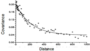
Spatial autocorrelation is present in all forests and has to do mainly with site factors and growth conditions that are highly correlated for trees that are close together and that are much lesser correlated for trees that are farther away from each other. The same holds also for sample plots: plots that are spatially close to each other tend to exhibit more similar values than those with a longer distance in between. Figure 1 gives an example; there, however, the covariance is given; as correlation is simply the standardized covariance, the shape of the function holds exactly also for the autocorrelation; for the autocorrelation the y-axis would need to be re-scaled to the range of 0.0 to 1.0. In that graph, the points mark measured covariances of various pairs of observations at the same distance. The line is then a smooth curve fitted to the observed values. The shape of the curve is typical: high correlation for observations that are close to each other (and an autocorrelation of 1.0 if the distance is 0, because then, the same object is observed twice), and constantly decreasing covariance (autocorrelation) with increasing distance. From a certain distance onwards a more or less steady level of no correlation is reached.
Relevance for plot design planning
First we state that we would like to design observation plots such that the within-plot variability is as high as possible. That means, per sample plot we wish to capture as much variability as possible. The reason is simple: the more variability we capture per plot the smaller will be the variability between the sample plots – and it is the variance between the plots that determines the error variance. High correlation means that by knowing one value we can fairly well predict the other value of the pair of observations. That means, if two variables are highly correlated, the added value of measuring the second variable is relatively low once the value of the first variable is known (because the value of the second variable can fairly well be predicted). And the same holds for autocorrelation: if the autocorrelation between the values of two objects is high then it is less beneficial (in terms of gain of information) to also measure the second object.
As a consequence of this consideration, from a statistical viewpoint of capturing as much information as possible per plot we wish to keep the autocorrelation between pairs of observed objects (trees or plots or …) low; and that means that we want to make the distances between the objects large.
References
- ↑ Kleinn, C. 2007. Lecture Notes for the Teaching Module Forest Inventory. Department of Forest Inventory and Remote Sensing. Faculty of Forest Science and Forest Ecology, Georg-August-Universität Göttingen. 164 S.