Estimating forest area
Contents |
Area estimation is among the very principal results of large area forest inventory. Estimation can be done for different categories such as forest and non-forest or different forest types. Forest area estimation is also a crucial input to all quantifications or estimations of “deforestation”. A clear definition of “forest” is required in any case.
For the determination of forest area there are at least two basic approaches:
- delineation (mapping) from remote sensing imagery, or
- Statistical sampling (either in the field or from remote sensing imagery).
Mapping can either been done automatically (in the presence of suitable algorithms) or manually. Various sources of error are associated with this exercise but the result is a map that shows the spatial arrangement of the forest patches. Statistical sampling is a different approach that produces an overall estimation – but not a map. It has the advantage that the precision in terms of the standard error is easily quantified (if statistical sampling has been used) and gives information about the reliability of the estimation.
Results of area estimations are given either in absolute (\(km^2\) or \(ha\)) or in relative term (%). Also, precision statements can be given either in absolute terms (standard error, confidence interval) or in relative terms (relative standard error, percent confidence interval). If a percent forest cover estimation is accompanied by a precision statement (for example 40% ± 5%) – then it is important to clearly state whether the precision statement is meant in absolute terms (in this case (35% ≤ cover ≤ 45%) or in relative terms (38% ≤ cover ≤ 42%); otherwise, confusions may easily occur.
Area estimation can be based on different plot designs that are discussed in what follows: points, lines and plots.
Area estimation by points
Points are dimensionless plots on which only a very limited set of observations can be made. Therefore, the observations are either yes or no for a set of area classes. For estimating forest area by sample points means that points are selected and for each point it is determined whether it comes to lie in forest or not; that makes the two possible observations \(y=1\) and \(y=0\), respectively. With these observed values, estimations are being carried out as for any other variable. Sample points may be selected at random, systematically, in clusters etc., just all sampling designs are possible. For area estimation, however, the most common approach is a dot grid; that is a systematic sample. The grid is randomly (random point and random orientation) placed over the area of interest and then it is simply counted how many points fall into forest; if, out of the total sample size n there are \(n_f\) forest points, then the forest cover proportion is estimated from
\[\hat{p}=\frac{n_f}{n}\,\]
this, actually, derives from the standard estimator of the mean for simple random sampling, assigning the observation \(y=1\) to the \(n_f\) forest points and the observation \(y=0\) to the \(n_n\) non-forest points.
Then
\[\hat{p}=\frac{\sum_{i}y_i}{n}=\frac{1}{n}\left(n_f*1+n_n*0\right)=\frac{n_f}{n}\,\]
As for systematic sampling in general, there is no unbiased estimator for the variance estimation. Therefore, we resort to the estimator framework of simple random sampling. There, we know that we may use the binomial distribution to calculate variances. The binomial distribution describes the outcome of “experiments” or observations of variables that can take on only two values (0 or 1, yes or no, black or white). If \(p\) is the true (parametric) proportion of target elements in the population (in our case: the forest cover), then the parametric population variance is
\[\sigma^2=p*q=p*(1-p)\,\]
where \(q=(1-p)\). The variance, obviously, is a function of the mean p only!
The variance \(\sigma^2=p*q\) derives directly from the formula used for calculating the population variance in general:
\[{\sigma_p}^2=\frac{\sum_{i}\left(y_i-\bar{y}\right)^2}{N}\,\]
where \(\bar{y}\) is the true proportion p and there are only two possibility of observations: (1) \(y=1\) for forest points which occur \(n_f\) times where
\[p=\frac{n_f}{N}\,\]
and \(y=0\) for non-forest points which occur \(n_n=(n-n_f)\) times and
\[q=\frac{n_n}{N}=\frac{N-n_f}{N}\,\]
We rewrite then
\[\sigma^2=\frac{\sum_{i}(y_i-\bar{y})^2}{N} =\frac{\sum_{i}(y_i-p)^2}{N}\frac{n_f(1-p)^2+n_n(0-p)^2}{N}\] \[=\frac{n_f}{N}(1-p)^2+\frac{N-n_f}{N}(0-p)^2=p(1-p)^2+(1-p)^2=p(1-p)=p*q\,\]
which is the parametric variance. The sample based estimation of that variance has \((n-1)\) degrees of freedom so that the sum of squares needs to be divided by \((n-1)\). We may use the same re-arrangement as before and care for the different denominator simply by introducing the factor \(\mbox{n/(n-1)}\)
\[s^2=\frac{\sum_{i}(y_i-\hat{p})^2}{n}*\frac{n}{n-1}=\hat{p}*\hat{q}*\frac{n}{n-1}\,\]
The estimated error variance of \(\hat{p}\) derives as usual from
\[\hat{var}(\hat{p})=\frac{s^2}{n}\,\]
which in this case is
\[\hat{var}(\hat{p})=\frac{\hat{p}\hat{q}}{n-1}\,\]

Observe that, contrary to the known error variance estimator for simple random sampling, here the denominator is \((n-1)\) and not n; this should not be confusing any more after the derivations presented.
Area estimation by dimensionless points on a map or on an aerial photograph is usually done as systematic sampling using a dot grid. One may imaging using a transparency sheet on which a dot grid is printed and this transparency sheet is placed randomly on the map of interest.
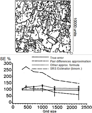
Here, we may illustrate the characteristics of systematic sampling. An illustration is in Figure 1: there, the forest area is estimated with dot grids of different sizes. The map is given in Figure 1, up; it has a side length of 10000 units. The size of the dot grids used for area estimation is measured in these units.
In Figure 1, the relative standard errors of different estimators are compared to the approximated true value which is set to 100% for all grid sizes. The true value was determined by a typical experiment, carried out as sample simulation in the computer: to determine the approximate true standard error of estimating the area in that particular map with a grid of a particular size (say 1000 units wide, which corresponds to an expected value of the sample size of n = 1000 in this case), such grid is superimposed very often randomly on the map. For each randomly placed dot grid we obtain an estimation for the area. After having repeated this sampling for, say, 5000 times (as was done in the simulations from which Figure 1, below, was produced) the approximated standard error of the estimated area derives directly as the standard deviation of these 5000 estimated values. The standard errors were determined for all grid sizes as depicted in Figure 1, below, and then set to 100% for comparison with other estimators.
Applying the simple random sampling estimator to the systematic sample (the dot grid), we systematically overestimate the true standard error (long dashed line in Figure 1, below). The overestimation is much more for denser grids (larger plot sizes): in this example, for a grid size of 500 units, the standard error for the random sample is about 3 times as large as the one for systematic sampling – and that is quite some difference. It means also that the same precision is being reached by a systematic sample with only about 1/3 of the sample size which has direct cost implications! For very wide grids (low sample size) the true standard error of systematic sampling and the one resulting from simple random sampling are fairly close. We may imagine (but not more!) that, for very wide dot grids, the sampling process resembles somewhat a systematic sample. The performance of systematic sampling in comparison to simple random sampling, however, does in this example also depend on the fragmentation structure of the landscape: the more fragmented the lesser superior is the systematic sample.
In Figure 1, below, there is also the comparison presented with the pair-differences technique and a second approximation formula. In this particular case, both are closer to the true value than the simple random sampling estimator. But this is not always so. For the pair-differences estimator in this example, there is a light overestimation for higher sample sizes and an underestimation for larger grid sizes. Only for the simple random sampling estimator it is known that it systematically and always overestimates so that we can be sure that we deal with a conservative estimation. This is probably one of the major reasons why it is preferred in many cases.
Area estimation by lines or clusters of points


Area estimation can be done by line intercept sampling where sample lines are used as observation units and on each sample line it is observed which proportion comes to.
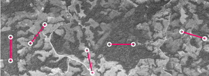
In Figure 2 two basic approaches are described for area estimation from such sample lines:
- standard line intercept sampling: in this case, the observation that is made on the line can take on all values between \(y=0.0\) and \(y=1.0\);
- observing only the end points of the line, so that clusters of two points are formed that are a defined distance away from each other: in this case, the observation that is made on one cluster can take on only three values \(y=0.0,\) \(y=0.5\) and \(y=1.0\).
Obviously, line intercept sampling takes more time to implement, because the measurement of the proportion of the line inside forest is time consuming. This is much faster when only the end points are observed. The effort is the same for all observation units completely outside or completely inside the forest (regardless whether it is line intercept sampling or sampling with clusters of points.
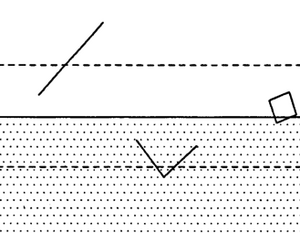
The comparison of precision of estimation is now of interest. In order to research into that, we may imagine simple situation as depicted in Figure 3 (from Kleinn 1991): the area consists of 50% forest and 50% non-forest, a straight line separates the two halves and we now wish to estimate the forest area with a sample line. In Figure 3, there are two other line sampling units depicted (a square and a half-square) which are not further discussed here. Because of the symmetry of this „map” it is sufficient to look at all positions of the sample line along a line that is perpendicular to the forest edge and extends through the buffer (between the dashed lines in Figure 3) where the buffer is defined such that a line has an intersection probability larger than 0 if its center point falls into it. All lines outside this buffer are either completely outside the forest \((y=0)\) or completely inside the forest \((y=1)\). Observe: the buffer as drawn Figure 3 is for the sample line; the buffer would be smaller for the L-shape and the square line sampling unit which are also depicted.
With geometric probabilities the true parametric mean and error variance of the area estimation can be determined. The mean, obviously, is always \(p=0.5\). The error variances are given in Table 1, for both the estimation from line intercept sampling (observing line sections) and from observing the cluster of end-points. For the line, this cluster consists of two points, for the L-shape (the half square) of three points and for the square of four points.
Table 1. Result of precision comparison of 2 area estimation approaches using sample lines. The error variances
refer to the population of all observation units within the buffer strip between the dashed lines in Figure 3 (Kleinn 1991[1]).
Variance would be \(\frac{1}{4}(\mapsto\sigma^2=p*q)\) for single independently selected sample points.
Observation unit Line intercept sampling Clusters of points Line
(2 points)\(\frac{1}{4}\approx0.14393\,\) \(\frac{1}{4}-\frac{1}{2\pi}\approx0.09085\,\) L-shape = half square
(3 points)\(\frac{1}{4}\frac{(1+\sqrt{2})}{6\pi\sqrt{2}}\approx0.12693\,\) \(\frac{1}{4}-(1+\sqrt{2})\frac{2}{9\pi}\approx0.07923\,\) Square
(4 points)\(\frac{1}{4}-\frac{3+\sqrt{2}5\ln(1+\sqrt{2})}{12\pi\sqrt{2}}\approx0.08455\,\) \(\frac{1}{4}-(1+\sqrt{2})\frac{1}{4\pi}\approx0.05788\,\)
It may be surprising, but the estimation from clusters of points is more precise: for the line shape, the line intercept sampling approach produces an error variance of
\[\sigma_{\hat{p}}^2=\frac{1}{4}-\frac{1}{3\pi}=0.14393\,\]
while the one for the clusters of two points is
\[\sigma_{\hat{p}}^2=\frac{1}{4}-\frac{1}{2\pi}=0.09085\,\]
It is more precise and less costly to do the area estimation from observations of points only rather then observing along the entire line. This holds for all three compared observation units: the simple sample line, the L-shape or half square and the square.
However, we must not generalize this observation, but need to restrict it to cases for which the simple model from Figure 3 applies, and this is cases in which one observation unit does not intersect with more than one forest boundary; that means: the observation units (the line sample elements used) are relatively short in comparison to the forest patches in the area of interest. In many large area forest inventories, this condition is fulfilled; for example, in the German NFI, square clusters of 150 m side length are used and the connecting line can be used as sample line. While in the first German NFI, line intercept sampling was applied to estimate the area proportion for the different forest types. However, it was found that the estimation via observation of the cluster corners only does yield equally precise area estimations so that line intercept sampling was abandoned for the second German NFI where only a cluster of four points was analyzed for area estimation.
Estimation of length from the estimation of areas
A special case shall be briefly presented here, where area estimation had been used to estimation the length of gallery forests in an inventory region. In a large area forest inventory in Costa Rica, the length of gallery forests was an issue (Kleinn et al. 2005[2]). Sample plots were laid out over the entire country, not only in forest but also in open lands. The objective was to carry out a tree inventory rather than a forest inventory only.
From the observations on sample plots in the field and in aerial photographs the gallery forest cover was estimated to be 2.2% of the country. This was actually a quite surprisingly high figure if one imagines that gallery forests are just narrow strips of forest. That figure alone underlines the overall relevance in that country of this forest type that has high relevance for biodiversity conservation, for water and soil protection (and, by the way, also for cattle farmers who have access to water almost everywhere!).
If we assume an average width of gallery forests of 50 m and a total land area of \(51,000km^2\) for Costa Rica, we may calculate an estimated length of the gallery forests: the \(2.2%\) of \(51,000km^2\) are an absolute area of \(1122km^2\) and if we imagine this area to be a strip of \(50m\) width, we obtain a rectangle of \(50m*22,440km\); the length of this rectangle corresponds then to the estimated total length of gallery forests. When determining the density of gallery forests, we need to take into account that they occur only outside other forest types, that is in the open landscape. In Costa Rica, the cover of non-forest + gallery forest area is \(51.6%+2.2%=53.8%\) and the gallery forest density is then estimated to be \(816m\) per square km \((22,400km/51,000km^2*0.538\)).
References
- ↑ 1.0 1.1 1.2 1.3 Kleinn C. 1991. Der Fehler von Flächenschätzungen mit Punkterastern und linienförmigen Stichprobenelementen. Dissertation. Mitteilungen der Abteilung für Forstliche Biometrie 91‑1, Universität Freiburg, 128 S.
- ↑ Kleinn C., C. Ramírez, P. Holmgren and G. Chavez. 2005. A national forest resources assessment for Costa Rica based on low intensity sampling. Forest Ecology and Management 210:9-23.