File list
This special page shows all uploaded files. When filtered by user, only files where that user uploaded the most recent version of the file are shown.
| Date | Thumbnail | Size | User | Description | Versions | |
|---|---|---|---|---|---|---|
| 13:34, 30 June 2015 | 2015-06-11 Power and politics Brockhaus.pdf (file) | 2.8 MB | Schreiner | 1 | ||
| 08:09, 17 September 2015 | 2 1 van tuyll.pdf (file) | 434 KB | Fehrmann | 1 | ||
| 08:23, 17 September 2015 | 2 2 miah&pardo villegas.pdf (file) | 2.28 MB | Fehrmann | 1 | ||
| 08:24, 17 September 2015 | 2 3 kabajani&singh.pdf (file) | 1.4 MB | Fehrmann | 1 | ||
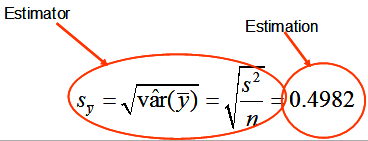
| 00:41, 10 March 2011 | 3.5-fig00.png (file) |  | 152 KB | Aspange | (The estimator is the calculation algorithm (formula) that produces the estimation. Reference: Kleinn, C. 2007. Lecture Notes for the Teaching Module Forest Inventory. Department of Forest Inventory and Remote Sensing. Faculty of Forest Science and Fores) | 1 |
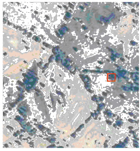
| 00:27, 10 March 2011 | 3.7-fig44.png (file) |  | 767 KB | Aspange | (Distribution of sample based estimations of deforestation for Bolivia with 10% sampling intensity. Left: a wide range of estimated deforestation figures is produced when the original 41 Landsat scenes are taken as population. However, when these 41 images) | 1 |
| 11:11, 17 September 2015 | 3 1 ham.pdf (file) | 2.78 MB | Fehrmann | 1 | ||
| 11:12, 17 September 2015 | 3 2 perez.pdf (file) | 3.91 MB | Fehrmann | 1 | ||
| 11:12, 17 September 2015 | 3 3 magdon.pdf (file) | 7.12 MB | Fehrmann | 1 | ||
| 12:17, 5 October 2015 | 3 4 schreiner&roux.pdf (file) | 944 KB | Fehrmann | 1 | ||
| 23:44, 9 March 2011 | 4.1.1-fig45.png (file) |  | 398 KB | Aspange | (Typical shape of a spatial autocorrelation function. Here, however, the covariance is given. The correlation would look exactly the same, but with a y-axis re-scaled to the range of 0.0 to 1.0. Reference: Kleinn, C. 2007. Lecture Notes for the Teaching ) | 1 |
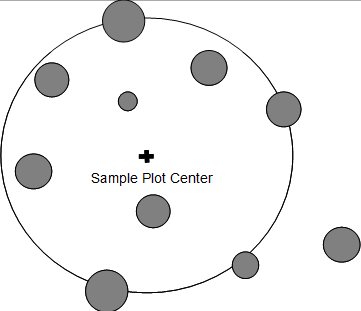
| 09:34, 3 March 2011 | 4.2.2-fig46.png (file) |  | 330 KB | Aspange | (With circular sample plots all trees are taken as sample trees that are within a defined distance (radius) from the sample point, which constitutes the plot center. Reference: Kleinn, C. 2007. Lecture Notes for the Teaching Module Forest Inventory. Depa) | 2 |
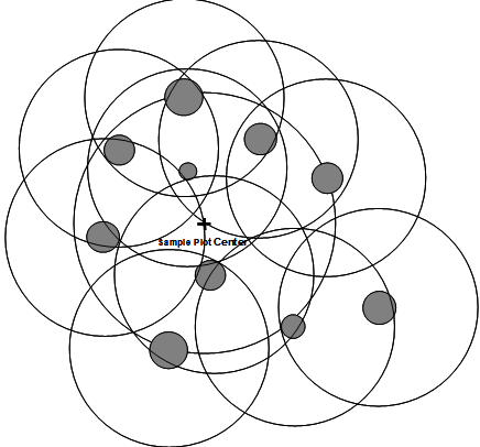
| 09:35, 3 March 2011 | 4.2.2-fig47.png (file) |  | 520 KB | Aspange | (Illustration of the inclusion zone approach: For fixed area circular plots, the inclusion zones are identical for all trees. Those trees are taken as sample trees in whose inclusion zones the sample point comes to lie. Reference: Kleinn, C. 2007. Lectur) | 2 |
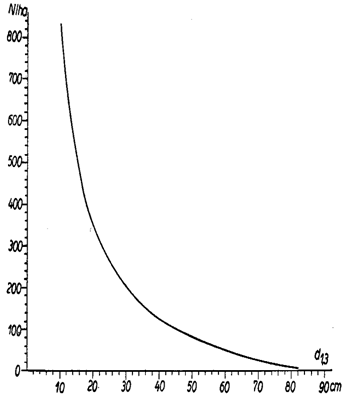
| 08:51, 3 March 2011 | 4.2.2-fig48.png (file) |  | 402 KB | Aspange | (Typical diameter distribution in a natural forest. Reference: Kleinn, C. 2007. Lecture Notes for the Teaching Module Forest Inventory. Department of Forest Inventory and Remote Sensing. Faculty of Forest Science and Forest Ecology, Georg-August-Universi) | 1 |
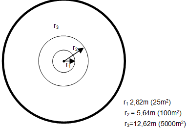
| 08:52, 3 March 2011 | 4.2.2-fig49.png (file) |  | 296 KB | Aspange | (Nested sub-plots showing 3 circular plots having different sizes, radii, but sharing same plot center Reference: Kleinn, C. 2007. Lecture Notes for the Teaching Module Forest Inventory. Department of Forest Inventory and Remote Sensing. Faculty of Fores) | 1 |
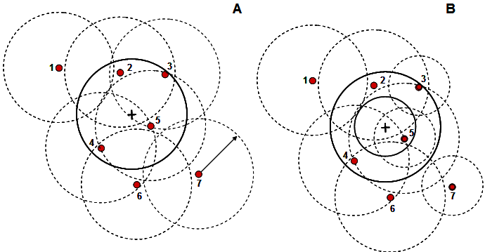
| 08:53, 3 March 2011 | 4.2.2-fig50.png (file) |  | 727 KB | Aspange | (Comparison of the inclu-sion zone approach for nested circular sub-plots (B) and for fixed circu-lar plots (A). Reference: Kleinn, C. 2007. Lecture Notes for the Teaching Module Forest Inventory. Department of Forest Inventory and Remote Sensing. Facult) | 1 |
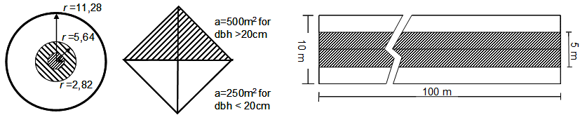
| 08:57, 3 March 2011 | 4.2.2-fig51.png (file) | 398 KB | Aspange | (Different combination of shapes for nested sub-plots. Reference: Prodan M., R. Peters, F. Cox and P. Real 1997. Mensura forestal. Serie investigación y educación en desarrollo sostenible. IICA/GTZ. 561p.) | 1 | |
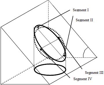
| 09:10, 3 March 2011 | 4.2.6-fig52.png (file) |  | 313 KB | Aspange | (A diagram showing an area of refer-ence and projected area into the map plane on a sloping terrain. Reference: Kleinn C., B. Traub and C. Hoffmann 2002. A note on the slope correction and the estimation of the length of line features. Canadian Journal o) | 1 |
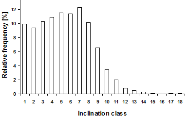
| 09:30, 3 March 2011 | 4.2.6-fig53.png (file) |  | 272 KB | Aspange | (Distribution of inclination of forest plots of the second Swiss National Forest Inventory (class 0, 0-9.99%, class 1, 10-19.99%, etc.) Reference: Kleinn C., B. Traub and C. Hoffmann 2002. A note on the slope correction and the estimation of the length ) | 1 |
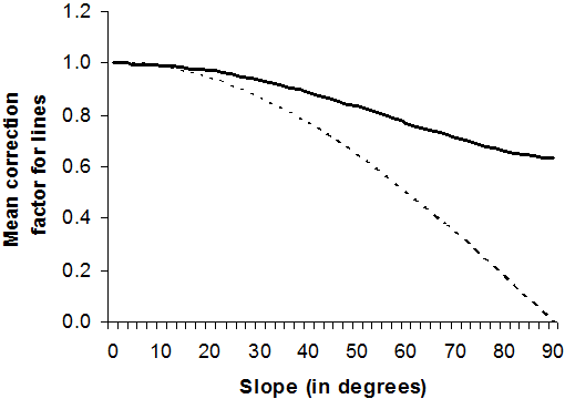
| 10:02, 3 March 2011 | 4.2.6.1-fig54.png (file) |  | 539 KB | Aspange | (Mean correction factor for line features as a function of terrain inclination a (bold line), assuming that the lines have a uniform distribution of angular deviation from the gradient vector. The dashed line gives the standard correction factor cos(<math>) | 1 |
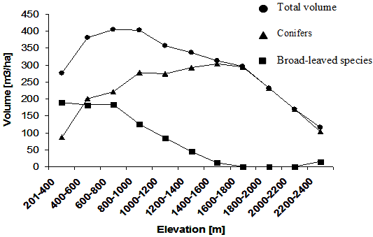
| 10:16, 3 March 2011 | 4.2.6.2-fig55.png (file) |  | 531 KB | Aspange | (Volume over elevation estimated from the second Swiss National Forest Inventory. Reference: Kleinn C., B. Traub and C. Hoffmann 2002. A note on the slope correction and the estimation of the length of line features. Canadian Journal of Forest Research 3) | 1 |
| 21:11, 5 March 2011 | 4.3-fig56.png (file) | 387 KB | Aspange | (Different techniques applied to boundary plots. Only the mirage technique is not causing a systematic error. From left to right: mirage method, shifting the plot, enlarging the circular plot at the same location such that the plot area is maintained, and ) | 1 | |
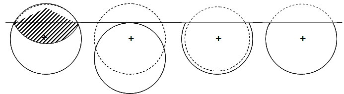
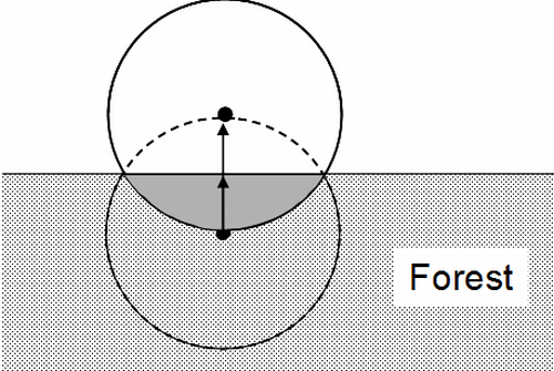
| 21:14, 5 March 2011 | 4.3-fig57.png (file) |  | 492 KB | Aspange | (Principle of the mirage method for border plot correction. The center of the plot is mirrored at the forest edge outside the forest. From that new point, again a circular plot is laid out and all trees tallied again which fall into it; these trees are obs) | 2 |
| 21:46, 5 March 2011 | 4.3-fig58.png (file) |  | 681 KB | Aspange | 2 | |
| 21:32, 5 March 2011 | 4.4.1-fig59.png (file) |  | 273 KB | Aspange | (Illustration of selection proportional to size (basal area) in Bitterlich sampling. Reference: Kleinn, C. 2007. Lecture Notes for the Teaching Module Forest Inventory. Department of Forest Inventory and Remote Sensing. Faculty of Forest Science and Fore) | 1 |
| 21:44, 5 March 2011 | 4.4.2-fig60.png (file) |  | 369 KB | Aspange | 2 | |
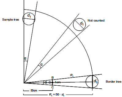
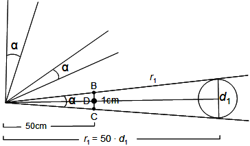
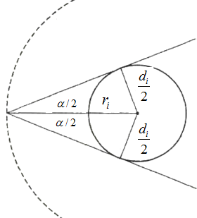
| 21:42, 5 March 2011 | 4.4.2-fig61.png (file) |  | 228 KB | Aspange | (Illustration of calculation of the radius of the virtual circular sub-plot for a tree with diameter <math>d_i</math>. Reference: Kleinn, C. 2007. Lecture Notes for the Teaching Module Forest Inventory. Department of Forest Inventory and Remote Sensing. ) | 1 |
| 22:32, 5 March 2011 | 4.4.2-fig62.png (file) |  | 254 KB | Aspange | (Critical angle principle. Reference: Kleinn, C. 2007. Lecture Notes for the Teaching Module Forest Inventory. Department of Forest Inventory and Remote Sensing. Faculty of Forest Science and Forest Ecology, Georg-August-Universität Göttingen. 164 S.) | 1 |
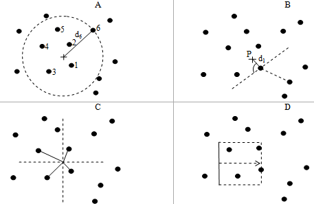
| 23:46, 7 March 2011 | 4.5.1-fig63.png (file) |  | 399 KB | Aspange | (Some variations of ''k''-tree sampling. Reference: Kleinn, C. 2007. Lecture Notes for the Teaching Module Forest Inventory. Department of Forest Inventory and Remote Sensing. Faculty of Forest Science and Forest Ecology, Georg-August-Universität Götti) | 1 |
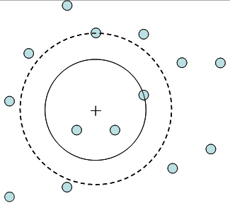
| 23:48, 7 March 2011 | 4.5.1-fig64.png (file) |  | 281 KB | Aspange | (Illustration why the simple expansion factor approach does produce a systematic overestimation for k-tree sampling. Reference: Kleinn, C. 2007. Lecture Notes for the Teaching Module Forest Inventory. Department of Forest Inventory and Remote Sensing. Fa) | 1 |
| 23:55, 7 March 2011 | 4.5.1-fig65.png (file) |  | 545 KB | Aspange | (Illustration why the simple expansion factor approach does produce a systematic overestimation for ''k''-tree sampling. Reference: Kleinn, C. 2007. Lecture Notes for the Teaching Module Forest Inventory. Department of Forest Inventory and Remote Sensing) | 1 |
| 00:19, 8 March 2011 | 4.5.3-fig66.png (file) |  | 372 KB | Aspange | 1 | |
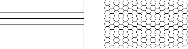
| 22:27, 9 March 2011 | 4.8-fig68.png (file) | 481 KB | Aspange | (Illustration of approach 1 for plot populations: subdivision of the forest area into sample plots of identical shape and size, here: square and hexagonal sample plots. Such a subdivision is also possible for rectangles and some types of triangles. Refere) | 1 | |
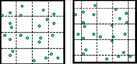
| 22:32, 9 March 2011 | 4.8-fig69.png (file) |  | 302 KB | Aspange | (An identical “forest area” subdivided in two different ways in square sample plots of the same basic size. Right: plot fragments occur along the border line. The total of “number of stems” is obviously identical in both cases; but this is not the ) | 1 |
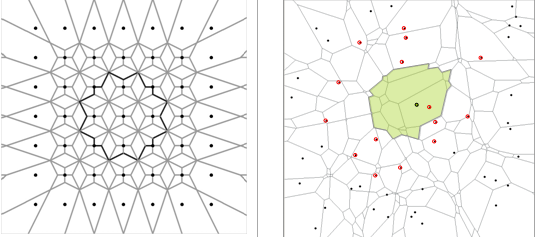
| 22:45, 9 March 2011 | 4.8-fig70.png (file) |  | 786 KB | Aspange | (Illustration of approaches for plot populations for the same example population. Left: discrete population of square sample plots with defined positions. Right: each point in the area is a sampling element the value of which is determined by the surroundi) | 1 |
| 11:16, 17 September 2015 | 4 1fehrmann.pdf (file) | 13.03 MB | Fehrmann | 1 | ||
| 11:16, 17 September 2015 | 4 2 dos santos&myint myat.pdf (file) | 2.08 MB | Fehrmann | 1 | ||
| 11:16, 17 September 2015 | 4 3 bustamante&kirgizbekova.pdf (file) | 1.38 MB | Fehrmann | 1 | ||
| 11:17, 17 September 2015 | 4 4 kukunda.pdf (file) | 3.19 MB | Fehrmann | 1 | ||
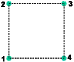
| 19:59, 16 December 2010 | 5.1.3-fig73.png (file) |  | 78 KB | Aspange | 1 | |
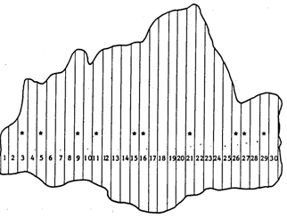
| 19:17, 16 December 2010 | 5.2.6-fig74.png (file) |  | 98 KB | Aspange | 1 | |
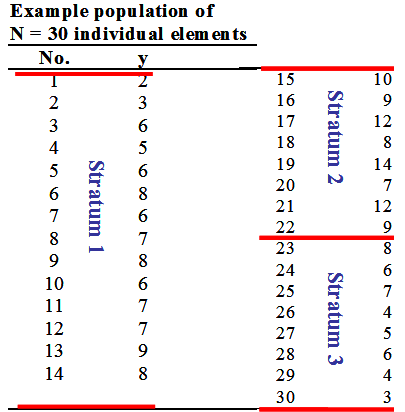
| 00:42, 30 December 2010 | 5.2.6-fig75.png (file) |  | 490 KB | Aspange | (Sub-dividing the example population (arbitrarily) in three strata, for illustration purposes. Reference: Kleinn, C. 2007. Lecture Notes for the Teaching Module Forest Inventory. Department of Forest Inventory and Remote Sensing. Faculty of Forest Scienc) | 8 |
| 21:15, 16 December 2010 | 5.3.4-fig81.png (file) |  | 19 KB | Aspange | (Cluster plot design as used in a regional forest inventory in the NOrthern Zone of Costa Rica (Kleinn 1993). This design is used to illustrate approaches to area estimation.) | 1 |
| 21:13, 10 December 2010 | 5.4-fig85.png (file) |  | 446 KB | Aspange | 1 | |
| 23:34, 10 December 2010 | 5.4-fig86.png (file) |  | 87 KB | Aspange | 1 | |
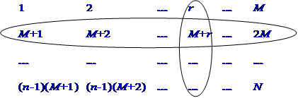
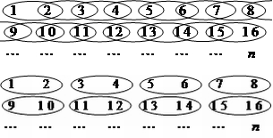
| 12:08, 22 December 2010 | 5.5.1-fig87.png (file) |  | 58 KB | Aspange | (Illustration of systematic sampling in terms of stratified sampling or cluster sampling. The population of <math>N</math> elements is arranged here in groups of <math>M</math>. Reference: Kleinn, C. 2007. Lecture Notes for the Teaching Module Forest Inv) | 1 |
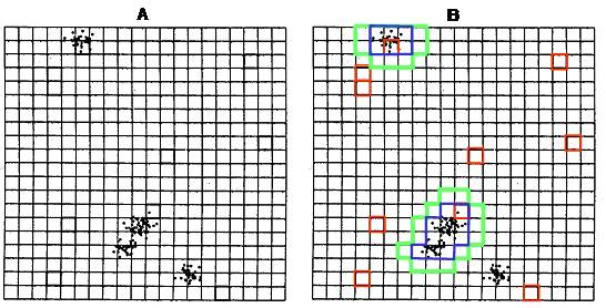
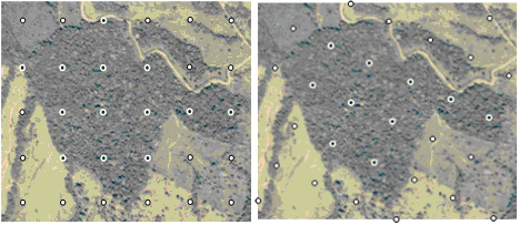
| 12:33, 22 December 2010 | 5.5.2-fig88.png (file) |  | 278 KB | Aspange | (One and the same grid randomly laid over the same area results in different numbers of sample points inside the forest area. Reference: Kleinn, C. 2007. Lecture Notes for the Teaching Module Forest Inventory. Department of Forest Inventory and Remote Se) | 1 |
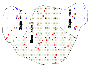
| 12:50, 22 December 2010 | 5.5.3-fig89.png (file) |  | 68 KB | Aspange | (When a population is sub-divided into strata, systematic sampling always produces proportional allocation of plots. Reference: Kleinn, C. 2007. Lecture Notes for the Teaching Module Forest Inventory. Department of Forest Inventory and Remote Sensing. Fa) | 1 |
| 13:07, 22 December 2010 | 5.5.5-fig90.png (file) |  | 314 KB | Aspange | (Two examples of the difference between random and fixed orientation grids. Left: squares of different side lengths (abscissa) are sampled with grid of unit size. Right: a forest map is sampled with random and fixed orientation grids of different width whe) | 1 |
| 13:12, 23 December 2010 | 5.5.6.4-fig91.png (file) |  | 139 KB | Aspange | (Building pairs of neighboring observations for the approximation of error variance in systematic sampling. Pairs can either be built “exclusively” (below) or overlapping (above). Reference: Kleinn, C. 2007. Lecture Notes for the Teaching Module For) | 1 |
First page |
Previous page |
 Next page |
Last page |