Creating jigsaw puzzles in ArcMap
(→The concept of cluster inclusionzones for fixed area sample plots) |
|||
| (40 intermediate revisions by 2 users not shown) | |||
| Line 1: | Line 1: | ||
| − | ==The concept of cluster | + | ==The concept of cluster selection zones for fixed area sample plots== |
| − | The so called '''jigsaw puzzle view''' (Roesch et al. 1993<ref name="roesch1993">Roesch, F.A.; Green, E.J.; Scott, C.T. 1993. An Alternative View of Forest Sampling. Survey Methodology 19 (2), 199-204.</ref>) is a | + | The so called '''jigsaw puzzle view''' (Roesch et al. 1993<ref name="roesch1993">Roesch, F.A.; Green, E.J.; Scott, C.T. 1993. An Alternative View of Forest Sampling. Survey Methodology 19 (2), 199-204.</ref>) is a tessellation of the total domain of interest in non-overlapping selection zones for exclusive clusters of trees. In the [[infinite population approach]] sample elements are dimensionless points drawn from an infinite [[Lecturenotes:Population|sample frame]]. On the other side we can only imagine a certain discrete number of possible observations derived over a number of nearest neighbors (trees) to a certain sample point. With fixed area [[sample plot]]s neighbors are included up to a fixed distance (the plot radius). This "inclusion distance" can be assigned to every tree in the domain of interest. Whenever a sample point falls in that distance it would lead to an inclusion of the respective tree in a sample. This single tree [[inclusion probability|inclusion zone]]s are overlapping (as in most cases more than only one tree is selected by a sample point) whereas the resulting pattern is a tessellation of the total area in non-overlapping polygons, that would lead to a selection of a particular cluster of trees. As the number of possible observations (derived from clusters of conjointly included trees) is much smaller than the infinite number of possible sample points, the jigsaw puzzle is a classification of the infinite sample frame in a finite number of areas of possible observations. This number of observations that can be obtained by sampling is the virtual [[Lecturenotes:population|population]] in which sampling is conducted. The size of the polygons is an expression of the [[inclusion probability|selection probability]] for a certain observation. |
| − | This article describes | + | This article describes, how jigsaw puzzles can be created from a map with tree locations in ArcGIS. |
===Workflow of creating jigsaw puzzles=== | ===Workflow of creating jigsaw puzzles=== | ||
| + | A tessellation of the area of interest can e.g. be obtained by means of GIS software. The following description refers to a simple model that can be implemented in ArcGIS and is able to derive a tesselation for circular sample plots. Basis for the calculation is the information about the [[inclusion probability]] of each spatially dispersed element that is derived based on the relation between a tree's inclusion zone and the total area of interest. Therefore trees are buffered with the radius of sample plots. | ||
| − | + | [[file:jigsawmodel.jpg|center]] | |
| − | [[ | + | |
| + | For each tree it is possible to calculate the number of trees/ha that it represents once it is included in a sample under the stipulated plot design. By intersecting all buffers one can tessellate the area in single polygons that are related to a certain combination of included trees and/or to a certain observation that can be made on this mutually exclusive set. By populating all single tree observations that are included by sample points in such a polygon, it is possible to calculate the resulting estimate of the number of trees/ha that would result at this point. | ||
| − | + | [[file:jigsaw.png|700px|center]] | |
| − | + | ||
| − | + | ===jigsaw puzzles for k-tree sampling=== | |
| − | + | In case of [[Distance based plots|k-tree sampling]] single trees are selected as most nearest neighbors to a sample point. In contrast to fixed area plots the neighborhood is not defined by a maximum inclusion distance (a certain fixed bandwidth) but is restricted to a fixed number of neighbors. Also in this case it is possible to create jigsaw puzzles. Same like in the example above they are a decomposition of the total domain of an infinite number of possible sample point locations in exclusive areas (polygons) for each particular realization that is possible based on the given spatial distribution of trees. Each polygon is composed by the infinite number of points that would lead to the selection of a particular cluster of k trees. The decomposition of the domain is a so called Voronoi diagram in case of k=1 and a higher order Voronoi diagram (kth order) in case that k neighbors are selected per sample point. | |
| − | + | The following example shows a Voronoi diagram for 6-tree sampling. | |
| − | + | ||
| − | + | ||
| − | + | ||
| − | + | ||
| − | + | ||
| − | === | + | |
| − | + | ||
| − | + | ||
| − | + | ||
| − | + | ||
| − | + | ||
| − | + | ||
| − | + | ||
| − | + | ||
| − | + | ||
| − | + | ||
| − | + | ||
| − | + | ||
| − | + | ||
| − | + | ||
| − | + | ||
| + | [[Image:k-treejigsaw.jpg|center]] | ||
| + | The number of polygons is equal to the number of all possible clusters with 6 nearest trees (all points inside one polygon would select the same cluster) and as result also the number of all possible realizations of a certain target variable. The area of single polygons is, if related to the total area, an expression of the selection probability of the observation derived from the related cluster. | ||
| + | Another point in this context is the determination of unbiased expansion factors for the selected trees. Therefore the inclusion probability of each single tree has to be derived. The inclusion area related to each tree is the number of all sample points, that would lead to a selection of the particular tree as cluster element. The tree is a cluster element in case that it is one of the k nearest neighbors to a sample point. | ||
[[Category:HowTo]] | [[Category:HowTo]] | ||
Latest revision as of 15:00, 25 October 2015
Contents |
[edit] The concept of cluster selection zones for fixed area sample plots
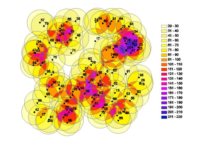
The so called jigsaw puzzle view (Roesch et al. 1993[1]) is a tessellation of the total domain of interest in non-overlapping selection zones for exclusive clusters of trees. In the infinite population approach sample elements are dimensionless points drawn from an infinite sample frame. On the other side we can only imagine a certain discrete number of possible observations derived over a number of nearest neighbors (trees) to a certain sample point. With fixed area sample plots neighbors are included up to a fixed distance (the plot radius). This "inclusion distance" can be assigned to every tree in the domain of interest. Whenever a sample point falls in that distance it would lead to an inclusion of the respective tree in a sample. This single tree inclusion zones are overlapping (as in most cases more than only one tree is selected by a sample point) whereas the resulting pattern is a tessellation of the total area in non-overlapping polygons, that would lead to a selection of a particular cluster of trees. As the number of possible observations (derived from clusters of conjointly included trees) is much smaller than the infinite number of possible sample points, the jigsaw puzzle is a classification of the infinite sample frame in a finite number of areas of possible observations. This number of observations that can be obtained by sampling is the virtual population in which sampling is conducted. The size of the polygons is an expression of the selection probability for a certain observation. This article describes, how jigsaw puzzles can be created from a map with tree locations in ArcGIS.
[edit] Workflow of creating jigsaw puzzles
A tessellation of the area of interest can e.g. be obtained by means of GIS software. The following description refers to a simple model that can be implemented in ArcGIS and is able to derive a tesselation for circular sample plots. Basis for the calculation is the information about the inclusion probability of each spatially dispersed element that is derived based on the relation between a tree's inclusion zone and the total area of interest. Therefore trees are buffered with the radius of sample plots.
For each tree it is possible to calculate the number of trees/ha that it represents once it is included in a sample under the stipulated plot design. By intersecting all buffers one can tessellate the area in single polygons that are related to a certain combination of included trees and/or to a certain observation that can be made on this mutually exclusive set. By populating all single tree observations that are included by sample points in such a polygon, it is possible to calculate the resulting estimate of the number of trees/ha that would result at this point.
[edit] jigsaw puzzles for k-tree sampling
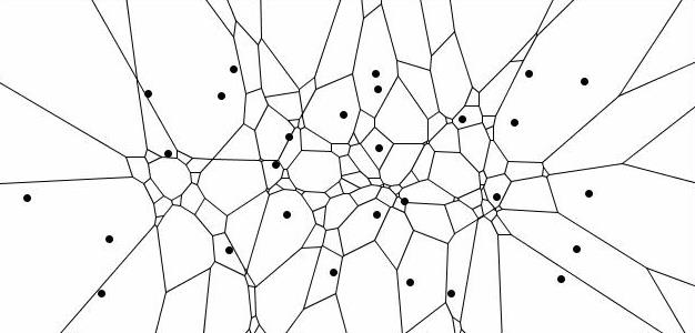
In case of k-tree sampling single trees are selected as most nearest neighbors to a sample point. In contrast to fixed area plots the neighborhood is not defined by a maximum inclusion distance (a certain fixed bandwidth) but is restricted to a fixed number of neighbors. Also in this case it is possible to create jigsaw puzzles. Same like in the example above they are a decomposition of the total domain of an infinite number of possible sample point locations in exclusive areas (polygons) for each particular realization that is possible based on the given spatial distribution of trees. Each polygon is composed by the infinite number of points that would lead to the selection of a particular cluster of k trees. The decomposition of the domain is a so called Voronoi diagram in case of k=1 and a higher order Voronoi diagram (kth order) in case that k neighbors are selected per sample point. The following example shows a Voronoi diagram for 6-tree sampling.
The number of polygons is equal to the number of all possible clusters with 6 nearest trees (all points inside one polygon would select the same cluster) and as result also the number of all possible realizations of a certain target variable. The area of single polygons is, if related to the total area, an expression of the selection probability of the observation derived from the related cluster.
Another point in this context is the determination of unbiased expansion factors for the selected trees. Therefore the inclusion probability of each single tree has to be derived. The inclusion area related to each tree is the number of all sample points, that would lead to a selection of the particular tree as cluster element. The tree is a cluster element in case that it is one of the k nearest neighbors to a sample point.
[edit] References
- ↑ Roesch, F.A.; Green, E.J.; Scott, C.T. 1993. An Alternative View of Forest Sampling. Survey Methodology 19 (2), 199-204.


