Line sampling

Forest Inventory lecturenotes

Category Forest Inventory lecturenotes not found

Introduction

Line sampling uses one-dimensional lines as observation units, just as we may use for many purposes fixed area sample plots (two-dimensional observation units) or points (dimensionless observation units). Line sampling does not refer to the so-called transects which usually mean elongated narrow strips, that is: two-dimensional plots. Depending on the dimensionality of the observation units, different types of observations can be made on them. There are three major applications of line sampling :

• It may be observed which portion of a sample line comes to lie in forest. These portions can be used to estimate the forest cover percent. This type of sampling is called line intercept sampling.

• It may be observed how many times a sample line intersects with a line feature in the landscape such as forest edges, roads or creeks. The number of intersections can be used to estimate the total length of these line features. This type of sampling is called line intersect sampling (LIS).

• It may be observed whether a population element is intersected or not by a sample line. By this, we may use the line samples to make a random selection of population elements in the absence of an a priori sampling frame.

A good reference for line sampling is deVries (1986) or earlier related studies by deVries.

To remember!

It is very easy to mix up the two different line sampling techniques. It is important to remember that Line Intercept Sampling is completely different from Line Intersect Sampling. While we just look at relative shares of line segments (here the observation units) inside a target class in Line Intercept Sampling, the second technique is applicable to estimate the length of linear features just by counting the intersections with the sample line.

Line intercept sampling

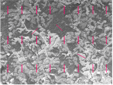
Line intercept sampling is used to estimate the cover of defined classes in the landscape, for example forest or forest types. Line samples are randomly placed over the area of interest and on each sample line it is observed which proportion comes to lie in the target area class. The observation per sample line can take on values between 0 and 1. From these observations, the mean, variance and error variance can be estimated along the known estimators. Line intercept sampling is typically applied in aerial photographs when rapid area estimations are desired. However it is also applied in the field: in large area forest inventory cluster sampling, one may use, for example, the connecting lines between sub-plots to do line intercept sampling. Figure 1 illustrates this approach by overlaying a systematic sample of equally oriented lines of n = 24 and a random sample of randomly located and randomly oriented lines of n = 3.

Figure 1. Application of line intercept sampling on an aerial photograph.

Let \(l_{i(in)}\) be the length of the sample line i which is inside the target condition class such as forest, \(l_{i(total)}\) be the total length of the sample line i; then, the observation \(y_i\) which is made on line i is

\[y_i = \frac {l_{i(in)}} {l_{i(total)}}\].

The estimated proportion \(\hat p\) in the region off interest is then estimated from n randomly placed sample lines from

\[\hat p=\frac {\sum_{i=1}^n y_i}{n}\]

and the variance in the population is estimated from

\[s^2=\frac {\sum_{i=1}^n (y_i - \hat p)^2}{n-1}\].

The error variance is \(s_p^2 = \frac {s^2}{n}\).

These estimators hold for simple random sampling and sample lines of the same length. It may be that sample lines have different length; for example if the lines cross the entire region of interest and are randomly placed. Then, the ratio estimator may be applied to increase the precision of estimation, using the length of the individual sample line as ancillary variable (see also sampling with unequal selection probability).

Line intersect sampling

The terms line intersect sampling and line intercept sampling should not be confused: line intersect sampling bases on counting intersections of the sample lines with line features in the landscape. It is obvious that there will be more intersections with line samples, the longer the line feature in the landscape is. By simply counting the intersections (and knowing the total length of the sample lines), one can then produce an estimation of the total length of the line feature. This is frequently used for the estimation of the length of the forest edge or for the length of the road network in a region of interest in which that sample line is located. Line intersect sampling goes back to an experiment from the 18th century:

Buffon’s needle problem (1777)

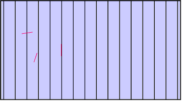
The French noble man Comte de Buffon researched into the basic questions: If a needle of length \(l_i\) is thrown randomly on an area completely covered by equidistant parallel lines with the distance W (and the line length \(l_i\) being shorter than W), what is the probability that the needle intersects with one of the parallels (This example is also known as Buffon's needle problem).

Figure 2. Illustration of Buffon´s needle problem: the probability is to be estimated that a needle intersects with one of the parallel lines.

This is illustrated in Figure 2. The solution follows the standard procedure when determining probabilities: we must try and define the size of the total population of needles and then identify that part of the population of needles that intersect with one of the parallels. The ratio of these two is the searched probability.

The motivation of Mr. Buffon was obviously to investigate the characteristics of gambling.

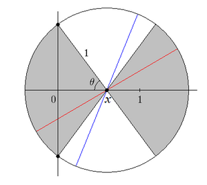
This problem can be solved by geometric probabilities and is illustrated in Figure 3 on the left, where we concentrate on only one of the parallels. After this, the position of a particular needle ee′ relative to the parallels is defined

• by the center point M of the needle and its distance m to the nearest parallel, and

• by the orientation, that is the angle φ between the orientation of the needle and the orientation of the parallels.

About the line shown in Figure 3, a rectangle is centered with the width W and the length L; remember W is the distance between the parallels and L is the total length of the parallel. Within this rectangle, only specific combinations of the above mentioned factors do lead to an intersection of the needle with the centered line. That means: as a function of these two factors, one can determine whether the needle intersects or not. The population of needles is defined by all points of the area of interest and for each point by all possible orientations; where the area of interest is formed by the rectangle WL. If the distance of the needle from the parallel is larger than \(l_i/2\), an intersection is not possible at all so that we can subdivide the area of interest from the outset in two domains: Needle positions nearer than \(l_i\) to the parallel (here, the intersection depends on the angle φ) and those farther away than li for which the intersection is impossible.

Because of symmetry it is sufficient to investigate what happens at one side of the perpendicular line, and it is sufficient to look at angles φ from 0 to 90°, or in radians from 0 to \(\frac {\pi}{2}\). Thus, it is imperative that

\[0 \le m \le \frac {l_i}{2}\] and \(0 \le \varphi \le \frac {\pi}{2}\),

where m and φ are stochastically independent variables and equally distributed in the correspondent intervals. We can now identify those combinations of m and φ for which an intersection takes place. To do so, let’s introduce the distance x between the midpoint M of the needle and the intersection point S (Figure 3, left), for which it is imperative that

The red and blue needles are both centered at x. The red one falls within the grey area, contained by an angle of 2θ on each side, so it crosses the vertical line; the blue one does not. The proportion of the circle that is grey is what we integrate as the center x goes from 0 to 1

\[x \le \frac {l_i}{2}\].

The variable x is a function of m and φ and can, thus, be replaced by

\[\frac {m}{sin \varphi}\]

what finally results in

\[m \le \frac{l_i}{2}sin(\varphi)\].

As a result, for all needle positions / combinations below the line

\[m = \frac{l_i}{2}sin(\varphi)\]

an intersection takes place (Figure 3 right). That graph can also be read as follows: imagine a fixed value for the distance \(m_x\), represented by a parallel to the abscissa passing through the value \(m_x\) at the y-axis; for all values of φ left to the intersection with the function, there is no intersection with the parallels, but there is intersection for all angles φ right to the intersection with the function.

Figure 3. Intersection probability as a function of the orientation of the needle and the distance of the needle to the nearest line (from deVries 1986)

Finally, the probability of intersection is the ratio of the dotted area and the total area. That total area is the rectangle with side length W/2 and \(\frac {\pi}{2}\); and the area of intersection is

\[A_{intersect} = \int_{\varphi=0}^{\frac {\pi}{2}}\, \frac {l_i}{2} sin(\varphi)\, d\varphi = \frac {l_i}{s}[-cos \varphi]_0^{\frac {\pi}{2}} = \frac {l_i}{2}\].

Thus, the probability of intersection of the needle with one of the parallels is given by the simple expression

\[\pi_{i1} = \cfrac {\cfrac{1}{2}l_i}{\cfrac {1}{2}\pi * \cfrac {1}{2}W} = \frac {2l_i}{\pi W}\]

Observe that this term holds only for an experimental arrangement like illustrated in Figure 2. If we are interested in placing sample lines on an area of interest in order to estimate certain population characteristics like in Figure 3 left, we need to take the probability into account that M is within the rectangle WL. This is simply given by \(\pi_{i2} = \)WL/A and the final probability of intersection is

\[\pi_i = \pi_{i1} * \pi_{i2} = \frac {2l_iL}{\pi A}\].

As expected, the probability of intersection depends on the density of sample lines, given by line length per area L/A, and the length of the needle \(l_i\). Note that the term \(\pi_i\) is used here to indicate so-called inclusion probabilities (see Horvitz-Thompson estimator), which must be distinguished from the number \(\pi\).

By re-arranging the latter formula we see that the total line length L can be determined by the number of intersections, resulting from \(\pi_i, l_i\) and A by

\[L = \frac {\pi_i \pi A}{2l_i}\],

where \(\pi\) needs to be identified experimentally. One may also imagine a simple experiment to empirically determine the value of \(\pi\) by simply counting the number of intersections:

\[\pi = \frac {2Ll_i}{\pi_i A}\].

Applications of line intersect sampling

Line intersect sampling is applied in forest inventory practice in particular for estimating the forest edge length and for estimating the length of forest roads. Matérn (1964) presented the line intersect sampling approach for the latter purpose and estimated total line length as line length per unit area with

\[\hat \tau = \frac {\pi Am}{2L}\],

where m is the number of intersections of sample lines and the target line feature This formula results directly from combining the above derived probability of intersection \(\pi_i\) with the so-called Horvitz-Thompson estimator, which is given by

\[\hat \tau = \sum \frac {y_i}{\pi_i}\]. When \(\pi_i\)

is replaced with the above given expression, a general estimator for estimating characteristics of line features with line intersect sampling is

\[\hat \tau = \frac {\pi A}{2L} \sum \frac {y_i}{l_i}\].

This estimator immediately results in the above given estimator from Matérn if we replace \(y_i\) with \(l_i\), which is the length of the needle or object intersected, respectively.

Using sample lines as sample selection tools

Sample lines may also be used as a tool for sample selection in the absence of a sampling frame. Imagine an aerial photograph with many isolated objects on it like shrubs, or pieces of woody debris on the forest floor. One could then number the shrubs and randomly select some (this would be building a sampling frame first and then do the random selection). However, we may also throw a sample line of defined length randomly onto the area and select the shrub that is being intersected by the line. If the objects (shrubs) have different sizes, then this is sampling with unequal selection probabilities where the selection probability has to do with the length of the sample line and the size and shape of the objects. Given the same area, an object will have a higher selection probability if it has a narrow elongated shape.

Figure 4. If line intersect sampling is used as a tool to select sample objects, a “needle” is to be defined on each object. Only intersection of the sample line with this needle leads to the selection of that object.

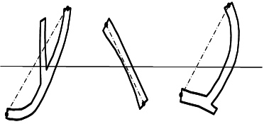
Following the basic features of line sampling and in order to make that approach operational, we define a “needle” on each element, a line that characterizes that object. Only if the sample line intersects with this needle, the object is going to be selected. Figure 98 illustrates that for the example of woody debris on the ground; again: not the intersection of the object with the sample line makes it to be selected, but the intersection with the needle defined on the object.

The length of the needle defines the inclusion probability of that particular object. If we measure the value of the target variable on each selected object, then we have the standard estimation situation of sampling with unequal selection probabilities. This technique is applied as standard element of sampling designs for down woody debris.

Following this, if we are interested in estimating the total volume of coarse woody debris on a given area of interest, one may apply the general estimator given in the preceding chapter. The only thing that has to be done is to determine the volume of the single logs intersected, what, for example, can be done with

Huber’s formula\[y_i = \frac {\pi}{4}d_i2 l_i\],

where \(d_i\) is the diameter at the point of intersection. Thus, the final estimator is

\[\hat \tau = \frac {\pi^2 A}{8L} \sum d_i^2\]

and only one diameter measurement per object is necessary.

An excellent and complete discussion of line intersect sampling with more fields of application can be found in the text book of Gregoire and Valentine (2008) in chapter 9.

simple

In this example line elements are used to select target objects in an area of interest. The target variable is not measured with or along the lines, but might be any other variable of interest measured on the selected objects. Following the above explanation it is possible to determine the inclusion probability of the object that have to be known for unbiased sampling with unequal selection probabilities.

References

- ↑ Kleinn, C. 2007. Lecture Notes for the Teaching Module Forest Inventory. Department of Forest Inventory and Remote Sensing. Faculty of Forest Science and Forest Ecology, Georg-August-Universität Göttingen. 164 S.
- ↑ 2.0 2.1 de Vries PG. 1986. Sampling Theory for Forest Inventory. Springer-Verlag Berlin. 399p.
- ↑ Matérn B. 1964. A method of estimating the total length of roads my means of a line survey. Studia Forestalia Fennica Suecica 18:68-70.
- ↑ Gregoire TG and HT Valentine. 2008. Sampling Strategies for Natural Resources and the Environment. Chapman and Hall / CRC. 474p.