Slope correction
| (8 intermediate revisions by 2 users not shown) | |||
| Line 1: | Line 1: | ||
| − | {{Ficontent}} | + | {{Ficontent}} {{video|link=https://youtu.be/InPERYNxQ0E}} |
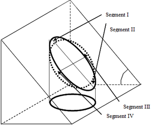
| + | [[File:4.2.6-fig52.png|right|thumb|300px|'''Figure 7''' A diagram showing an area of reference and projected area into the map plane on a sloping terrain (Kleinn et al 2002<ref name="kleinn2002">Kleinn C., B. Traub and C. Hoffmann 2002. A note on the slope correction and the estimation of the length of line features. Canadian Journal of Forest Research 32(4):751-756.</ref>).]] | ||
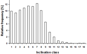
| + | [[File:4.2.6-fig53.png|right|thumb|300px|'''Figure 8''' Distribution of inclination of forest plots of the second Swiss National Forest Inventory (class 0, 0-9.99%, class 1, 10-19.99%, etc.)(Kleinn et al 2002<ref name="kleinn2002">Kleinn C., B. Traub and C. Hoffmann 2002. A note on the slope correction and the estimation of the length of line features. Canadian Journal of Forest Research 32(4):751-756.</ref>).]] | ||
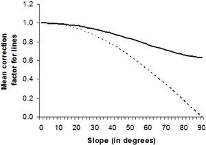
| + | [[File:4.2.6.1-fig54.png|right|thumb|300px|'''Figure 9''' Mean correction factor for line features as a function of terrain inclination <math>\alpha</math> (bold line), assuming that the lines have a uniform distribution of angular deviation from the gradient vector. The dashed line gives the standard correction factor cos(<math>\alpha</math>)(Kleinn et al 2002<ref name="kleinn2002">Kleinn C., B. Traub and C. Hoffmann 2002. A note on the slope correction and the estimation of the length of line features. Canadian Journal of Forest Research 32(4):751-756.</ref>).]] | ||
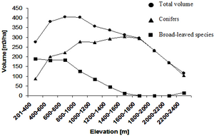
| + | [[File:4.2.6.2-fig55.png|right|thumb|300px|'''Figure 10''' Volume over elevation estimated from the second Swiss National Forest Inventory (Kleinn et al 2002<ref name="kleinn2002">Kleinn C., B. Traub and C. Hoffmann 2002. A note on the slope correction and the estimation of the length of line features. Canadian Journal of Forest Research 32(4):751-756.</ref>).]] | ||
==Slope correction== | ==Slope correction== | ||
| − | Results from forest inventories are area-related; examples are [[ | + | Results from forest inventories are area-related; examples are [[volume|volume/ha]], [[basal area|basal area/ha]], [[density|number of stems/ha]]. The area to which these measures refer is the [[map area]]; that is the horizontal projection of the terrain into the [[map plane]]. If we lay out a circular [[sample plot]] with a defined radius on the slope, the projected area in the map plane will be different. This is obviously not desired but if we wish to make an extrapolation of the per-plot observation to the per hectare observation, then '''all''' related areas must refer to the same reference system, and that is the map plane. |
As a consequence, if we have a defined [[plot area]] that is to be used for all sample plots, this area is defined in the map plane. If plots are to be laid out in sloped terrain, the plot area on the slope must be larger such that the target plot area results when the plot is horizontally projected. This is illustrated for circular fixed area plots in Figure 7. | As a consequence, if we have a defined [[plot area]] that is to be used for all sample plots, this area is defined in the map plane. If plots are to be laid out in sloped terrain, the plot area on the slope must be larger such that the target plot area results when the plot is horizontally projected. This is illustrated for circular fixed area plots in Figure 7. | ||
| Line 8: | Line 12: | ||
:<math>\frac{r}{\mbox{cos }\alpha}\,</math> | :<math>\frac{r}{\mbox{cos }\alpha}\,</math> | ||
| − | + | ||
If we do not have the possibility of making [[automatic correction]], another way of slope correction must be applied. The idea is to find the radius of the circle that has an area equal to the one of the ellipse. By that, we guarantee that the plot has the target area when projected into the map plane; by this procedure, we accept that the plot as projected into the map plane has an ellipse shape. | If we do not have the possibility of making [[automatic correction]], another way of slope correction must be applied. The idea is to find the radius of the circle that has an area equal to the one of the ellipse. By that, we guarantee that the plot has the target area when projected into the map plane; by this procedure, we accept that the plot as projected into the map plane has an ellipse shape. | ||
| Line 35: | Line 39: | ||
{{info | {{info | ||
|message=Info | |message=Info | ||
| − | |text=The angle <math>\alpha\,</math> refers to degree! If a slope angle is given in % it has to be converted to degree before (for e.g. 30% slope the angle in degree is calculated as arctan( | + | |text=The angle <math>\alpha\,</math> refers to degree! If a slope angle is given in % it has to be converted to degree before (for e.g. 30% slope the angle in degree is calculated as arctan(30/100)=16.7 degree)! |
}} | }} | ||
| Line 47: | Line 51: | ||
===Slope correction for line features=== | ===Slope correction for line features=== | ||
| − | In some inventories, also linear features are measured (or like in [[line sampling]] are used as [[Sampling design and plot design|observation unit]], like length of roads; length of water (creeks); and length of [[Forest Boundary|forest boundary]]. In principle, we can proceed like with all other variables: observing what we find on the plot and use the expansion factor to extrapolate to the whole of the inventory region (or to a per-hectare-estimate). However, in sloped terrain, the correct correction procedure must obviously be different from the described general slope correction, because the actual projected length of a line feature at the slope is a function of the actual slope of the line itself which is not the overall slope of the terrain! | + | In some inventories, also linear features are measured (or like in [[line sampling]] are used as [[Sampling design and plot design|observation unit]]), like length of roads; length of water (creeks); and length of [[Forest Boundary|forest boundary]]. In principle, we can proceed like with all other variables: observing what we find on the plot and use the expansion factor to extrapolate to the whole of the inventory region (or to a per-hectare-estimate). However, in sloped terrain, the correct correction procedure must obviously be different from the described general slope correction, because the actual projected length of a line feature at the slope is a function of the actual slope of the line itself which is not the overall slope of the terrain! |
The projection of an individual line segment must be based on its actual inclination. Application of any gross correction factor to all sampled line segments would not be correct. However, if no information on the orientation of the individual line segments is available; one may want to employ a mean correction factor, if we assume that the lines are uniformly distributed over all possible directions. | The projection of an individual line segment must be based on its actual inclination. Application of any gross correction factor to all sampled line segments would not be correct. However, if no information on the orientation of the individual line segments is available; one may want to employ a mean correction factor, if we assume that the lines are uniformly distributed over all possible directions. | ||
| Line 65: | Line 69: | ||
===Example: Slope correction with fixed area plots=== | ===Example: Slope correction with fixed area plots=== | ||
| + | {{info | ||
| + | |message=Info | ||
| + | |text=The angle <math>\alpha\,</math> refers to degree! If a slope angle is given in % it has to be converted to degree before (for e.g. 30% slope the angle in degree is calculated as arctan(0.3)=16.7 degree)! | ||
| + | }} | ||
| − | Suppose, we measure a 1000 m² fixed area plot on a slope of 30% and we count 10 trees in that plot. Without correcting for slope, we calculate an expansion factor of 10 and the estimation is 100 trees per hectare. | + | Suppose, we measure a 1000 m² fixed area plot on a slope of 30% (=16.7 degree) and we count 10 trees in that plot. Without correcting for slope, we calculate an expansion factor of 10 and the estimation is 100 trees per hectare. |
However, the 1000 m² plot on the slope (''r''=17.84''m'') becomes an ellipse when projected to the map plane with the two radii <math>r_1=17.84m</math> and <math>r_2=17.088m=r_1*\mbox{cos }\alpha</math> and an area of | However, the 1000 m² plot on the slope (''r''=17.84''m'') becomes an ellipse when projected to the map plane with the two radii <math>r_1=17.84m</math> and <math>r_2=17.088m=r_1*\mbox{cos }\alpha</math> and an area of | ||
| Line 81: | Line 89: | ||
{{info | {{info | ||
| − | |message= | + | |message=Observe! |
| − | |text= | + | |text=Please observe that we are not correcting the radius of a sample plot (like explained above) but assume that a plot of 1000m² was installed on the slope. Therefore we here correct the result. Don't confuse the two different approaches (and respective formulas)! |
}} | }} | ||
| + | |||
| + | |||
==References== | ==References== | ||
Latest revision as of 09:36, 12 March 2021


Contents |
[edit] Slope correction
Results from forest inventories are area-related; examples are volume/ha, basal area/ha, number of stems/ha. The area to which these measures refer is the map area; that is the horizontal projection of the terrain into the map plane. If we lay out a circular sample plot with a defined radius on the slope, the projected area in the map plane will be different. This is obviously not desired but if we wish to make an extrapolation of the per-plot observation to the per hectare observation, then all related areas must refer to the same reference system, and that is the map plane.
As a consequence, if we have a defined plot area that is to be used for all sample plots, this area is defined in the map plane. If plots are to be laid out in sloped terrain, the plot area on the slope must be larger such that the target plot area results when the plot is horizontally projected. This is illustrated for circular fixed area plots in Figure 7.
If we define (Figure 7) the target plot area in the map plane, then this plot becomes an ellipse when projected in the oblique plane, and this ellipse has a larger area than the original plot in the map plane. If electronic range finders that can also measure slope angle are used for distance measurement, then this ellipse can easily be laid out in the field where the two radii of the ellipse are automatically calculated. If \(r\) is the radius of the original plot in the map plane and \(\alpha\) the slope angle, then the two radii of the ellipse are \(r\) and
\[\frac{r}{\mbox{cos }\alpha}\,\]
If we do not have the possibility of making automatic correction, another way of slope correction must be applied. The idea is to find the radius of the circle that has an area equal to the one of the ellipse. By that, we guarantee that the plot has the target area when projected into the map plane; by this procedure, we accept that the plot as projected into the map plane has an ellipse shape.
Let´s assume that the circular sample plot has the defined area (in the plane)
\[F_p={\pi}r^2\,\]
If projected to a slope with slope angle \(\alpha\), an ellipse results with radii \(r\) and
\[\frac{r}{\mbox{cos }\alpha}\,\]
which has the area (on the slope),
\[F_{slope}=\pi r\frac{r}{\mbox{cos }\alpha}=\frac{\pi r^2}{\mbox{cos }\alpha}\,\]
This is larger than the one in the map plane. We wish now to find the radius \(r_{slope}\) of the circle that has that area and we find it as
\[r_{slope}=\frac{r}{\sqrt{\mbox{cos }\alpha}}\,\]
That means: in sloped terrain, the original plot radius needs to be multiplied by the slope correction factor
\[\frac{1}{\sqrt{\mbox{cos }\alpha}}\,\]
By that, a larger circle is generated which has an area equal to the area to the ellipse that would result if we projected the original plot size into the map plane. The correction factor is obviously always larger than 1.
 Info
Info
- The angle \(\alpha\,\) refers to degree! If a slope angle is given in % it has to be converted to degree before (for e.g. 30% slope the angle in degree is calculated as arctan(30/100)=16.7 degree)!
For application in forest inventories, slope correction factors are usually pre-calculated and tabulated. Alternatively, it is programmed in the field computers.
The slope correction is commonly applied for slopes larger than 10%. For smaller slopes the deviation is so small that it is accepted without correction.
Slope correction is in particular relevant, when inventorying forests in hilly and mountainous regions. Figure 8 illustrates that for the National Forest Inventory of Switzerland. There, only about 10% of the sample plots are in terrain with slopes less than 10%, and a considerable percentage (around 5%) are even on slopes with more than 100% inclination!
[edit] Slope correction for line features
In some inventories, also linear features are measured (or like in line sampling are used as observation unit), like length of roads; length of water (creeks); and length of forest boundary. In principle, we can proceed like with all other variables: observing what we find on the plot and use the expansion factor to extrapolate to the whole of the inventory region (or to a per-hectare-estimate). However, in sloped terrain, the correct correction procedure must obviously be different from the described general slope correction, because the actual projected length of a line feature at the slope is a function of the actual slope of the line itself which is not the overall slope of the terrain!
The projection of an individual line segment must be based on its actual inclination. Application of any gross correction factor to all sampled line segments would not be correct. However, if no information on the orientation of the individual line segments is available; one may want to employ a mean correction factor, if we assume that the lines are uniformly distributed over all possible directions.
The correction line in Figure 9 was derived numerically, it is approximated by
\[\mbox{cos}^2\frac{\alpha}{2.1}\,\]
It assumes uniform angular distribution of the orientation of line segments relative to the slope gradient. It gives good results for the range of slopes that matter for forest inventories, where the deviation from the numerically derived values is less than 1% for inclinations
\[0\le\alpha\le60°\,\]
[edit] Effects of slope correction
Concern is some time expressed that the usual slope correction ‑ that, while maintaining the target plot area, changes the shape of the plot from the correct ellipse to a larger circle ‑ introduces a systematic error in particular in cases where the target variable has a gradient along the slope gradient; then, more “average” elements will be observed (in segment III and IV of Figure 7) in the size-adjusted circle in the field, and lesser observations are made along the gradient (that is, in segments I and II). In fact, there are variables that change with altitude, i.e. have a gradient along the slope. Figure 10 illustrates that for volume per hectare as a result from the Swiss National Forest Inventory (here, it is interesting to note the difference between coniferous and broadleaved species). Although the gradient is significant, however, it is too small to be relevant in the context of the slope correction. For volume/ha, at least, we do not expect the slope correction to cause problems.
[edit] Example: Slope correction with fixed area plots
 Info
Info
- The angle \(\alpha\,\) refers to degree! If a slope angle is given in % it has to be converted to degree before (for e.g. 30% slope the angle in degree is calculated as arctan(0.3)=16.7 degree)!
Suppose, we measure a 1000 m² fixed area plot on a slope of 30% (=16.7 degree) and we count 10 trees in that plot. Without correcting for slope, we calculate an expansion factor of 10 and the estimation is 100 trees per hectare.
However, the 1000 m² plot on the slope (r=17.84m) becomes an ellipse when projected to the map plane with the two radii \(r_1=17.84m\) and \(r_2=17.088m=r_1*\mbox{cos }\alpha\) and an area of
\[F_E={\pi}r_1r_2=957.8m^2=1000m^2*\mbox{cos }\alpha\,\]
Where, the factor of 10 is valid for all plots on slopes less than 10%, the correct expansion factor for the 1000 m² circle at 30% has to be larger, as the circle becomes a smaller ellipse when projected to the map plane. The calculation is as follows:
\[\frac{10000m^2}{1000m^2}*\mbox{cos }\alpha=\frac{10000}{957.8}=10.44\,\]
and the correct estimation for the number of trees per hectare is:
\[104.4=100*\frac{1}{\mbox{cos }\alpha}\,\]
 Observe!
- Please observe that we are not correcting the radius of a sample plot (like explained above) but assume that a plot of 1000m² was installed on the slope. Therefore we here correct the result. Don't confuse the two different approaches (and respective formulas)!
[edit] References
- ↑ 1.0 1.1 1.2 1.3 Kleinn C., B. Traub and C. Hoffmann 2002. A note on the slope correction and the estimation of the length of line features. Canadian Journal of Forest Research 32(4):751-756.