Comparison of plot designs

[−] Forest inventory

[+] Introduction to forest inventory

[+] Forest mensuration

[+] Introduction to sampling

[+] Plot design

[+] Sampling design

[+] Estimation issues

[+] Planning issues

[+] UNFCCC Implications for Forest Monitoring

[+] Forest Inventory Examples

  Forest Inventory Glossary

This section is largely based on the paper Kleinn and Vilcko (2006a).

In forest inventory planning one needs to define the plot type to be used. In many cases there are traditions and conventions and not much is thought about the choice of the plot type.

The different plot types (1) fixed area plots, (2) Bitterlich plots and (3) distance based plots carry different practical issues of implementation but also different statistical properties. Here, we wish to look at the statistical properties and illustrate them with a simulation study. A tree map of from the Miombo woodlands in Northern Zambia served as sampling frame. As all tree positions were exactly known by their grid coordinates, simulation of different plot design could be carried out. There, 4969 trees were mapped on an area of 13.44 ha (369.72 trees/ha) with a basal area per hectare of 16.37 m²/ha.

In this simulation study, we compared sampling with fixed area plots, Bitterlich sampling and distance-based plots. Target variables were density (number of stems per hectare) and basal area per hectare. For the distance-based methods we used the empirical estimators (see distance-based plots) presented in Kleinn and Vilcko (2006a) and Eberhardt (1967), whereas the first listed one was rated as the most consistently best performer by Magnussen et al. (2008).

Figure 1a. Comparison of the performance of fixed area plots, Bitterlich plots and distance-based plots for the same sampling efforts each. The case study is based on one test stand of about 13.4 ha. k is the average number of trees that are expected per plot. Here: estimation of basal area per hectare; below: estimation of number of stems per hectare.

Figure 1b.

In order to make the plot types comparable in terms of expected field effort, we compared k-tree sampling with both fixed area circular plots and relascope plots that do, on average, yield k trees per sample point. With 369.72 trees per hectare in our maps, the fixed plot area a_k for an expected number of k trees per sample plot is

\[a_k = \frac{k}{369.72} * 10000 m^2\]

For relascope sampling, the basal area factor \(baf_k\) was defined such that the expected number of counted trees is k, that is

\[baf_k = \frac {16.37}{k} \frac {m^2}{ha}\]

For each plot design estimator we calculated the estimated variance \(S_p^2\) from a random sample of size 10000; the variance of the expanded per hectare values of these 10000 samples was taken as an approximation of the parametric variance \(\sigma_p^2\). The variance of the estimated mean \(\bar y\) for a random sample of a given size n follows then from

\[var(\bar y)=\frac{S_p^2}{n}\]

For relascope sampling and fixed area sampling unbiased estimators are known: the expected value is equal to the parametric value and statistical performance can be immediately described by the variance of the estimated mean values. However, for the k tree sampling estimators there is a difference between the expected value and the true parametric value (bias) and, consequently, the variance of the estimated means characterizes their variability around the biased expected value, not around the true parametric mean.

For a proper comparison of statistical performance, however, the variability about the true parametric mean is of interest so that the bias must also be taken into account; this is usually done by calculating the root mean square error(Cochran 1977):

\[RMSE=\sqrt{var(\bar y)+bias^2}\]

In order to make results comparable, we follow here the approach also applied by Picard et al.(2005) and use relative values, expressing both standard error and bias relative to the true parametric values: if \(\theta\) denotes the true parametric value and \(\hat \theta\) the estimate, then the standardized root squared error sRE is

\[sRE=\sqrt{\left(\frac{\sqrt{var(\hat \theta)}}{\theta}\right)^2+\left(\frac{E(\hat \theta)-\theta}{\theta}\right)^2}\]

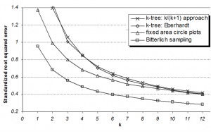
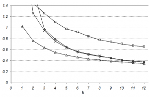
For an unbiased estimator sRE is identical to the relative standard error. Only the first term in that formula is a function of sample size, the bias remains the same even for large samples. That makes a comparison of biased and unbiased estimators difficult because they are differently affected by sample size. We use the simulation based variances \(S_p^2\) as an approximation for \(var(\hat \theta)\) in the above for comparison of the statistical performance of the plot designs. Results for the comparison are depicted in the Figure for plot sizes with k=1...12 trees each for basal area and for number of stems per hectare, respectively.

For basal area, relascope sampling produced the most precise results for all studied maps – which is not a surprise because this plot design selects individual trees proportional to the target attribute basal area. This superiority does also hold for larger k-values. Fixed area plots produce the next most precise results, while the difference between fixed area circle plots and the k-tree sampling estimators decreases with increasing k-values.

For estimation of density, however, the comparison of statistical performance yields different results: there, relascope sampling performs worst for all studied maps and for all k values; this can again be explained by the fact that relascope sampling is optimized towards basal area estimation, and not density (selection probabilities are proportional to size). These results are from but one stand, a generalization is not possible. But the basic characteristics of the different plot designs should hold for many other forest structures as well. One conclusion is: depending on the variable to be sampled, different plot types can be optimal. For basal area estimation there is no match to Bitterlich sampling which is clear because in that case trees are selected from each sample point proportional to the target variable basal area. However, the performance of Bitterlich sampling for estimating the number of stems is bad. In forest inventory, where many variables are to be observed per field plot, it is probably best to combine different plot types, as done, for example in the Finnish and the German national forest inventories. If one wants to stick to one single plot type, fixed area plots are probably the most consistently good performers over a wider range of variables.

References

- ↑ 1.0 1.1 Kleinn C. and F Vilčko. 2006a. A new empirical approximation for estimation in k-tree sampling. Forest Ecology and Management 237(2):522-533.
- ↑ Eberhardt LL. 1967. Some developments in distance sampling. Biometrics (23):207-216.
- ↑ Magnussen S, C Kleinn and N Picard. 2008. Two new density estimators for distance sampling. European Journal of Forest Research 127:213-224.
- ↑ Cochran, W., G., 1977. Sampling techniques. John Wiley & Sons
- ↑ Picard N, AM Kouyaté and H Dessard. 2005. Tree Density Estimations Using a Distance Method in Mali Savanna. Forest Science 51(1):7-18.