Simple random sampling
Contents |
General observations
Simple random sampling (SRS) is the basic theoretical sampling technique. The sampling elements are selected as an independent random sample from the population. Each element of the population has the same probability of being selected. And, likewise, each combination of n sampling elements has the same probability of being eventually selected.
Every possible combination of sampling units from the population has an equal and independent chance of being in the sample.
Simple random sampling is introduced and dealt with here and in sampling textbooks mainly because it is a very instructive way to learn about sampling; many of the underlying concepts can excellently be explained with simple random sampling. However, it is hardly applied in forest inventories because there are various other sampling techniques which are more efficient, given the same sampling effort.
For information about how exactly sampling units are choosen see Random selection.
Notations used
Estimators Parametric Sample Mean \(\mu = \frac{\sum_{i=1}^N y_i}{N}\) \(\bar {y} = \frac{\sum_{i=1}^n y_i}{n}\) Variance \(\sigma^2 = \frac{\sum_{i=1}^N (y_i - \mu)^2}{N}\) \(s^2 = \frac{\sum_{i=1}^n (y_i - \bar {y})^2}{n-1}\) Standard deviation \(\sigma = \sqrt{\frac{\sum_{i=1}^N (y_i - \mu)^2}{N}}\) \(s = \sqrt{\frac{\sum_{i=1}^n (y_i - \bar {y})^2}{n-1}}\) Standard error (without replacement or from a finite population)
\(\sigma_{\bar {y}} = \sqrt{\frac{N-n}{N-1}}*\frac {\sigma}{\sqrt{n}}\) \(S_{\bar {y}} = \sqrt{\frac{N-n}{N}}*\frac{S_y}{\sqrt{n}}\) Standard error (with replacement or from an infinite population)
\(\sigma_{\bar {y}} = \frac{\sigma}{\sqrt{n}}\) \(S_{\bar {y}} = \frac{S_y}{\sqrt{n}}\)
Where,
- \[N =\!\] number of sampling elements in the population (= population size);
- \[n =\!\] number of sampling elements in the sample (= sample size);
- \[y_i =\!\] observed value of i-th sampling element;
- \[\mu =\!\] parametric mean of the population;
- \[\bar {y} =\] estimated mean;
- \[\sigma =\!\] standard deviation in the population;
- \[S =\!\] estimated standard deviation in the population;
- \[\sigma^2 =\!\] parametric variance in the population;
- \[s^2 =\!\] estimated variance in the population;
- \[\sigma_{\bar {y}} =\] parametric standard error of the mean;
- \[s_{\bar {y}} =\] estimated standard error of the mean.
Examples
Example 1:
In this section, SRS estimators are illustrated with an example. This example will be pursued through the entire Lecture notes and illustrates that different sampling designs perform differently for the same population and with the same sample size.
The example population has \(N = 30\) individual elements; we may imagine 30 strip plots that cover a forest area (Figure 73). This dataset will also be used in the further chapters for comparison among the performance of different sampling techniques.
Table 11 lists the values of the 30 units. Here, for SRS, we are only interested in the y values. The \(x\) values are a measure for the size (area) of the strips; this will later be used in the context of other estimators.
From this population we get the following parametric values:
\(\mu = \frac{\sum_{i=1}^N y_i}{N} = 7.0667\) and \(\sigma^2 = \frac{\sum_{i=1}^N (y_i - \mu)^2}{N} = 7.1289\)
If we take samples of size \(n=10\), then the parametric error variance of the estimated mean is:
\(var (\bar {y}) = \frac {N-n}{N-1} * \frac {\sigma^2}{n} = 0.491645\)
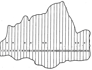
- Figure 1: Example population

- Table 1:Example Population of N = 30 individual elements
Number y x 1 2 50 2 3 50 3 6 100 4 5 100 5 6 125 6 8 130 7 6 130 8 7 140 9 8 140 10 6 130 11 7 140 12 7 150 13 9 160 14 8 170 15 10 180 16 9 200 17 12 210 18 8 210 19 14 210 20 7 200 21 12 200 22 9 180 23 8 160 24 6 140 25 7 120 26 4 90 27 5 90 28 6 100 29 4 100 30 3 80 Mean 7.0667 13950 Pop. variance 7.1289 2087.25
This value will be compared in the subsequent chapters with the error variances produced by other sampling techniques with the same sample size \(n=10\). The square root of the error variance is the standard error; and this is the true parametric standard error which we strive to estimate from a single sample then. To recap: the parametric standard error is the standard deviation of all possible samples of size \(n=10\). In a concrete sampling study, we have only one single sample of size \(n=10\) and from this sample the standard error can only be estimated.
Example 2:
Let´s take one single sample of \(n=10\) from the population of \(N=30\) given in Figure 1 and Table 1. Assume that the following elements were randomly selected:
Number \(y_i\) 3 6 5 6 9 8 11 7 15 10 16 9 21 12 26 4 27 5 29 4
We take now these ten selected sampling elements to produce estimations of the population parameters of interest. The estimated mean, variance in the population and error variance are, respectively:
\(\bar y = \hat {\mu} = 7.1 m^3\)
\(s^2 = \hat \sigma^2 = 6.9889\)
\(v\hat {a}r (\bar y) = 0.4659 = \frac {N-n}{N} * \frac {s^2}{n} = fpc \frac {s^2}{n}\)
Observe, that all estimated values differ from the true parametric values. In practice, however, we will never come to know how much this deviation actually is because the parametric values remain unknown.
However, we can make a probabilistic statement about the range in which we expect the true value to be; which is the confidence interval. For the estimated mean, the confidence interval is calculated from the estimated standard error and an assumption about the distribution of the sample means which is reflected in the value of the t-distribution. Accepting an error probability of \(\alpha = 5%\) that our statement is wrong, the width of one side of the confidence interval is:
\(t_{\alpha,v}S_{\bar y} = 2.262*0.6826 = 1.5440\) and then \(P(5.5560 < \mu < 8.6440)\,\!\).
This reads: the probability that the true parametric mean is in the interval between 5.556 and 8.644 is 0.95; it may however be that the true parametric mean is smaller or larger; this is the error probability of \(\alpha = 5%\). The given t-value can be read from tables or calculated from functions that usually every statistical software has built in. The actual values are depending on the degrees of freedom and the chosen error probability.
One may also calculate the confidence interval for the estimated variance in the population; which we do not here
The above sample has a size of n=10 and a sampling intensity of f = 10/30*100 = 33%. Here, sampling intensity can be calculated in terms of number of sampling units. Usually, however, the sampling intensity in forest inventories is calculated in terms of
\(f = \frac {total\, area\, of\, all\, sample\, plots}{total\, area\, of\, inventory\, region}\)
Estimation of the total: The estimator of the total is
\(\hat \tau = N * \bar y\), here\[\hat \tau = N * \bar y = 30 * 7.1 m^3 = 213\],
and the estimated variance of the estimated total is
\(v{\hat a}r(\hat \tau) = N^2\,v{\hat a}r(\bar y) = 30^2 * 0.4659 = 419.31\).