Cluster sampling

Introduction

Cluster Sampling (CS) is here presented as a variation of sampling design as it is done in most textbooks as well. However, in strict terms it is not a sampling design but just a variation of response design:

The major point in cluster sampling is that for each random selection of a sampling element not only one single sampling element is selected but a set (cluster) of sampling elements; thus, a cluster consists of a group of observation units, which together form a sampling unit. The selection itself (sampling design) can be done according to any sampling design (simple random, systematic, stratified etc.). Cluster sampling can be applied to any type of sampling element. If, on a production belt of screws one screw is selected randomly and the next 5 are also taken, then this set of 6 screws forms one observation unit consisting of 6 screws, because only one randomization (selection of the first srew) had been done to select this observation unit of 6. In fact, most basic plot designs as used in forest inventory can be viewed as cluster plots, where the cluster consists of a number of individual trees (this holds for fixed area plots, for Bitterlich plots etc.). In large area forest inventory, it is common that not single compact plots are laid out at each sample point but clusters of sub-plots. There, sub-plots are laid out in various geometric shapes and distances between them.

The above figure shows clusters with different geometric spatial arrangements of sub-plots. Each dot depicts one sub-plot. It is important to understand that the entire set of sub-plots is the observation unit or cluster (better: the cluster-plot).

It is important in this context to realize and understand that the entire cluster is one observation unit and the sample size is determined by the number of clusters and not by the number of sub-plots.

Info

This does often cause confusion but it is easy: we may call the entire cluster a cluster-plot; where the plot does not come in one compact piece (as with a circular fixed area plot) but is sub-divided into various distinct pieces. A cluster-plot can thus be viewed as a “funny shaped” plot.

It is a good terminology practice to always refer to “plot” if we talk about independently selected observation units. Therefore, the entire cluster is the plot (also called cluster-plot), and not the sub-plot. By erroneously referring to sub-plots as plots, one may cause confusion that may also lead to severe confusion about estimation as well.

Coming back to an example, in the following figure the basic principle of cluster sampling is illustrated based on a population of 48 elements that is grouped into N=24 clusters of size m=2. In cluster sampling, this population of clusters constitutes the sampling frame from which sample elements are drawn. With each random selection a set of two individual elements is drawn which, however, does produce but one observation for estimation. That means the total or mean of the two elements (that is: an “aggregated” value) and not the two individual values is then further processed for estimation.

It has been mentioned that cluster plots, consisting of m sub-plots are standard in large area forest inventory, such as many National Forest Inventories.

• 

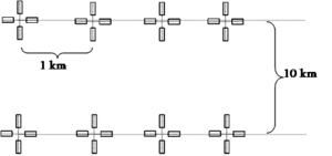
  Example of systematically arranged cluster plots.

• 

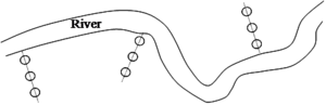
  clusterdesign with 3 circular sub-plots along a river.

• 

  Cluster sampling design in a forest fire area in East Kalimantan (Schindele 1989)

Notation

As with stratified sampling, some notation needs to be introduced when developing the estimators for cluster sampling:

Notation
\(L\,\)	Number of strata \(h=1, ... , L \,\)
\(N\,\)	Total population size = number of clusters in the population
\(M\,\)	Numberof sub-plots in the population \(M\sum_{i=1}^N m_i\,\)
\(\bar M\,\)	Mean cluster size in the population, \(\bar M=\frac{N}{M}\)
\(n\,\)	Sample size = number of clusters in sample
\(m_i\,\)	Number of sub-plots in cluster i, i.e. cluster size
\(\bar m\,\)	Mean cluster size in the sample
\(y_i\,\)	Observation in cluster i, i.e. total over all sub-plots of cluster i
\(\bar y_i\)	Mean per sub-plot in cluster plot i = \(\bar y_i = \frac {y_i}{m_i}\)
\(\bar y_c\,\)	Estimated mean per cluster in the sample = \(\bar y_c = \frac{1}{n} \sum_{i=1}^n y_i\)
\(\bar y\,\)	Estimated mean per sub-plot in the sample = \(\bar y = \frac{1}{n} \sum_{i=1}^n \bar y_i\)

Cluster sampling estimators

Clusters may have the same size m for all clusters or variable size \(m_i\). Obviously, this needs to be taken into account in estimation. In this section, we present the estimator for the situation of cluster-plots of equal size under random sampling. When the population consists of clusters of unequal size, then the ratio estimator will likely yield more precise results, because the ratio estimator uses the cluster size as ancillary variable.

sorry:

This section is still under construction! This article was last modified on 11/9/2010. If you have comments please use the Discussion page or contribute to the article!

References

- ↑ Schindele, W. 1989. Field Manual for Reconnaissance Inventory on Burned Areas, Kalimantan Timur. FR-Report No.2.