Bitterlich sampling

Forest Inventory lecturenotes

Category Forest Inventory lecturenotes not found

Introduction to angle count sampling

Figure 1 Illustration of selection proportional to size (basal area) in Bitterlich sampling (Kleinn 2007).

Angle count sampling was developed by Walter Bitterlich (1948), an Austrian forester. It is some times also referred to point sampling, horizontal point sampling, variable plot sampling, angle count technique, prism cruising, angle gauge sampling, and simply Bitterlich sampling.

The idea to employ nested sub-plots was introduced because we wished to have a balanced number of trees in all dimension classes; that is, we wanted to assign a higher probability of selection to the larger trees of which there are usually less in a stand (see also sampling with unequal selection probabilities).

For nested sub-plots, we defined a number of fixed plot areas in which the different dimension classes are observed. One may now further pursue that idea and develop a plot design in which the inclusion probability is strictly proportional to dimension. That is each tree has its particular and own plot size (and therefore also its particular inclusion zone). This is exactly what Bitterlich sampling does: from a selected sample point, the neighboring trees are selected strictly proportional to their basal area.

While this sounds complicated, the technique itself is very simple; the only device one needs is one that produced a defined opening angle. That can be a dendrometer, a relascope or simply your own thumb. While standing on the sample point and aiming over e.g. the thumb at the stretched out arm to the dbhs of the surrounding trees; you sweep around 360° and count all trees that appear larger than your thumb. It is obvious then, that larger trees have a larger probability of being taken as sample tree. From this counting alone you can produce then an estimate of basal area per hectare.

The only additional information that you need is the “calibration factor” of your measurement device, as, obviously, the number of trees counted depends on the opening angle which is produced by the instrument (in this case by your arm length and thumb width).

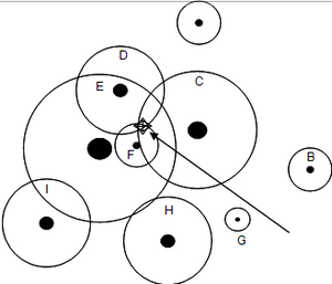
This calibration factor is also called basal area factor. Figure 1 illustrates that approach. Around each tree the individual inclusion zone is drawn. Sample points that fall into this inclusion zone will lead to an inclusion of this particular tree as sample tree. We may also imagine that these specific circular inclusion zones are concentrically placed around the sample point; then we may view them as a set of nested sample sub-plots, one for each sample tree.

Bitterlich sampling on sloped terrain

As in fixed area plot sampling, all area measures in angle count sampling are assumed to be in the map plane. When applying Bitterlich sampling in sloped terrain we need to take the slope into account; either by using an instrument that does the correction automatically, or by introducing the correction factor into the analysis if the slope is not automatically corrected (which is the case, for example, if using a stick with a panel, or the thumb); this slope correction is then to be applied from slopes of 10% and more. The correction factor is

\[\frac{1}{\cos\alpha}\,\]

so that the basal area per hectare observation from one Bitterlich sample point is

\[G_i=k*N_i\frac{1}{\cos\alpha_i},\,\]

where \(G_i=\) corrected basal area (\(m^2/ha\)) at the \(i^{th}\) sampling point, \(N_i=\) number of trees tallied at the sampling point and \(\alpha_i=\) angle of slope at the \(i^th\) sampling point.

The principle of Bitterlich sampling

Figure 2 The principle of Bitterlich sampling. For each tree, there are the three depicted situations (after Kramer & Akca 1995).

Figure 2 Illustration of calculation of the radius of the virtual circular sub-plot for a tree with diameter \(d_i\) (Kleinn 2007).

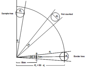
In a first step of developing this technique we need to calculate the size of these tree‑specific virtual sample plots. For each tree it holds the statement that it is only counted if it appears at 1.3 m larger than the opening angle of the measurement device. For each tree there are exactly three different situations as depicted in Figure 2: (1) either the tree is larger than the opening angle; then the tree is inside the virtual nested sub-plot and is counted; or (2) the tree is smaller than the opening angle (that is: completely covered by the thumb); that is a non-tally tree which is outside the virtual plot; or (3) the tree is exactly covered by the opening angle; then, the tree is exactly on the perimeter line of the virtual circular plot and the distance from the sample point to the center of that tree is (for practical purposes sufficiently good approximation to) the radius of the virtual circular plot. We need to find this radius, because the virtual plot will allow us to calculate the tree-specific expansion factor that we need to expand the per-plot observation to the per-hectare observation.

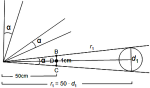
The opening angle can be produced by means of a stick of length c and a horizontal panel of width 1 cm at the end (analogous to arm and thumb, for example). For the virtual circle plot, for which this angle covers exactly a tree of dbh \(d_i\) (Figure 2) as a borderline tree, we obtain (approximately) plot radius \(r\) and plot area \(F_i\) along:

\[\frac{d_i}{r_i}=\frac{1}{c}\]

and then

\[r=cd_i\,\];

\[F_i={\pi}r^2={\pi}c^2{d_i}^2.\,\]

This is then the virtual plot in which all trees with exactly the dbh \(d_i\) are tallied.

This corresponds exactly to the procedure with nested circular plots where also only a defined size class was observed in each nested sub-plot. If we count \(n_i\) trees with exactly the diameter \(d_i\) (or in diameter class \(d_i\) in case that we work with diameter classes) at a sample point, then these trees have the basal area

\[{n_i}{g_i}=n_i\frac{\pi}{4}{d_i}^2.\,\]

Now, let’s expand this per-plot observation to a per-hectare figure (referring to trees with dbh \(d_i\) only!): the expansion factor is \(10000/F_i\), as usual, where \(F_i\) is the area of the virtual plot. The basal area per hectare for the trees of diameter \(d_i\) is then

\[G_{iHa}=\frac{10000}{F_i}n_i\frac{\pi}{4}{d_i}^2=\frac{10000}{\pi^2{d_i}^2}n_i\frac{\pi}{4}{d_i}^2=\frac{2500}{c^2}n_i.\,\]

Subsequently, this is done for all dbh-”classes” \(d_i\) and summed up to produce the estimate for the total basal area per hectare comprising all \(d\) classes:

\[G_{iHa}=\sum_{i}G_i=\frac{2500}{c^2}\sum_{i}n_i=\frac{2500}{c^2}N;\,\]

where \(G_{Ha}\) = basal area per hectare of all trees. The only variable in that equation is

\[N=\sum_{}n_i,\,\]

the number of observed/counted trees on the plot (over all diameter classes). This number of counted trees is multiplied with the factor

\[\frac{2500}{c^2}\,\]

which converts eventually the mere count into a basal-area-per-hectare value. This factor is called basal area factor and commonly denoted with \(k\). It is a factor that depends exclusively on the opening angle which is used.

By simply counting the \(N\) trees that are wider than our opening angle we can therefore produce an observation of basal area per hectare from a sample point:

\[G_{Ha}=k*N.\,\]

It must be observed, however, that only basal area per hectare can be observed as simple as that. For all other variable that may be of interest (such as mean diameter or number of stems), in addition the dbhs of all trees need to be measured. That is explained further below.

Basal area factors can be different. Table 1 gives the lengths \(c\) of this stick for basal area factors of 1,2,3 and 4 when there is a panel of 1 cm at the end of a that stick. Following the above formula, the length of that stick is calculated by

\[c=\frac{50}{\sqrt{k}}.\,\]

Table 1 Length \(c\) of the stick with 1cm for different values of the basal area factor \(k\)
Basal area factor (\(m^2/ha\))	c-value
\(k=1m^2\,\)	\(50\,\)
\(k=2m^2\,\)	\(35.4\,\)
\(k=3m^2\,\)	\(28.9\,\)
\(k=4m^2\,\)	\(25.0\,\)

Exact solution

Figure 4 Critical angle principle (Kleinn 2007).

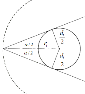
The principle presented above is, of course, only approximately correct, because the distance between the points at the tree where the viewing beams touch the tree is not exactly the tree diameter. For a geometrically correct calculation we would need to take that into account. The true distance between these two points is always shorter than \(d_i\). Figure 4 illustrates that and is gives the basis for the following calculations.

From Figure 4 we have

\[\mbox{sin }\frac{\alpha}{2}=\frac{\frac{d_i}{2}}{r_i}\,\]

and

\[r_i=\frac{d_i}{2*\mbox{sin }\frac{\alpha}{2}}.\,\]

The area of the virtual circular plot for the tree with diameter \(d_i\) is

\[A=\pi*r^2=\pi\frac{{d_i}^2}{4\left(\mbox{sin }\frac{\alpha}{2}\right)^2}\,\]

and the basal area per hectare results then from

\[G_i=10000*\frac{n_i*\frac{\pi}{4}*{d_i}^2}{\pi* \frac{{d_i}^2}{4*\left(\mbox{sin }\frac{\alpha}{2}\right)^2}}=10000*n_i*\left(\mbox{sin }\frac{\alpha}{2}\right)^2.\,\]

Basal area per hectare (of all trees) is then

\[G_{ha}=1000*\left(\sin\frac{\alpha}{2}\right)^2*\sum_{i=1}^k n_i,\,\]

where,

\[10000*\left(\sin\frac{\alpha}{2}\right)^2=k(\mathit{\mbox{basal area factor}}).\,\]

Therefore,

\[\sin\frac{\alpha}{2}=\frac{\sqrt{k}}{100}.\,\]

This is the mathematically correct derivation. However, the differences to the approximate solution as given above are so small that they can be accepted. The following gives the results of the simplified approximate calculation of the length \(c\) and the correct value \(c_c\):

\(k=1m^2\,\)	\(c_c=49.997\,\)	instead of	\(c=50\,\)
\(k=2m^2\,\)	\(c_c=35.352\,\)	instead of	\(c=35.355\,\)
\(k=4m^2\,\)	\(c_c=24.995\,\)	instead of	\(c=25\,\)

Anyway, for all the calculations, we need to make the assumption that the tree’s cross section is a perfect circle; which it is not; so that there are more sources of geometrical inaccuracies than the one described here.

Choice of basal area factor

The choice of the basal area factor (\(k\)) in Bitterlich sampling is equivalent to the choice of plot size for fixed radius plot sampling. The criteria to be considered in the choice of basal area factor are visibility in the stand and average number of sample trees desired at a sample point. A decrease in the basal area factors increases the average number of sample trees tallied in. But that means also that trees at a farther distance to the sample point will be tally-trees. This will work smoothly only when visibility is accordingly

In high density stands higher BAF values such as \(4 m^2/ha\) are used. In low density stands with good visibility, low BAF values such as \(1 m^2/ha\) is normally used. In temperate and boreal regions basal area factors of 1 or 2 are common; in dense tropical rainforest values of \(9 m^2/ha\) may be appropriate.

Of course, the target precision of a sampling study is always also an issue. With smaller values of \(k\) there will be more trees per sample plot (which comes together with somewhat higher cost) and with the same sample size, one will produce a higher precision than for larger values of \(k\).

Bitterlich sampling on sloped terrain

As in fixed area plot sampling, all area measures in angle count sampling are assumed to be in the map plane. When applying Bitterlich sampling in sloped terrain we need to take the slope into account; either by using an instrument that does the correction automatically, or by introducing the correction factor into the analysis if the slope is not automatically corrected (which is the case, for example, if using a stick with a panel, or the thumb); this slope correction is then to be applied from slopes of 10% and more. The correction factor is

\[\frac{1}{\cos\alpha}\,\]

so that the basal area per hectare observation from one Bitterlich sample point is

\[G_i=k*N_i\frac{1}{\cos\alpha_i},\,\]

where

\(G_i=\,\)	corrected basal area (\(m^2/ha\)) at the \(i^{th}\) sampling point
\(N_i=\,\)	number of trees tallied at the sampling point and
\(\alpha_i=\,\)	angle of slope at the \(i^{th} sampling point. |} ==Inclusion probabilities and estimators for Bitterlich sampling== For the inclusion zone approach where for each tree an inclusion zone is defined, see the corresponding article [[Infinite population approach]]. If used,the [[inclusion probability]] is then proportional to the size of this inclusion zone – which actually defines the probability that the correspondent tree is included in a sample. We saw, for example, that angle count sampling ([[Bitterlich sampling]]) selects the trees with a probability proportional to their [[basal area]] and we emphasized that this fact makes [[Bitterlich sampling]] so efficient for basal area estimation. In contrast, point to tree [[distance sampling]], or k-tree sampling, has inclusion zones that do not depend on any individual tree characteristic but only on the spatial arrangement of the neighboring trees; therefore, point-to tree distance sampling is not particularly precise for any tree characteristic. In [[Bitterlich sampling]], the selection probability of a particular tree ''i'' results from the inclusion zone ''Fi'' and the size of the reference area, for example the hectare UNIQ363fd09c1ad729b-MathJax-22-QINU with the Horvitz-Thompson estimator, we have the total UNIQ363fd09c1ad729b-MathJax-23-QINU for any tree attribute <math>y_i\). Applied to estimating basal area \(y_i = g_i = \frac {\pi}{4} d_i^2\) and its per hectare estimation, we have \[\hat \tau = \sum_{i=1}^m \frac {y_i}{\pi_i} = \sum_{i=1}^m \cfrac {\cfrac {\pi}{4} d_i^2}{\cfrac {F_i}{10000}}\] and with \( F_i = \pi r_i^2 = \pi c^2 \, d_i^2\), we have the same as Bitterlich sampling \[\hat \tau = \sum_{i=1}^m \frac {y_i}{\pi_i} = \sum_{i=1}^m \cfrac {\cfrac {\pi}{4} d_i^2}{\cfrac {\pi c^2 \, d_i^2}{10000}} = \frac {2500 \pi}{\pi c^2} \sum_{i=1}^m \frac {d_i^2}{d_i^2} = \frac {2500}{c^2} m\] which is the estimated basal area per hectare from one sample point where m trees were tallied. The factor 2500/c² is the basal area factor, for details see Bitterlich sampling. References