Volume functions

sorry:

This section is still under construction! This article was last modified on 03/1/2011. If you have comments please use the Discussion page or contribute to the article!

Forest mensuration lecture notes

[+] Definitions in forest inventory

[+] Functions and models in forest inventory

[+] Measurement devices

[+] Single tree variables

[+] Stand variables

  3D- Terrestrial laser scanning

  Forest Inventory Glossary

General observations

Volume functions are statistical models that describe the relationship between tree volume (dependent variable, to be predicted) with dbh, some times in combination with other variables such as tree height or an upper stem diameter. Before modeling volume as a function of one or more predictor variables, the variable “volume” needs to be defined. It is frequently defined as total {stem volume from the felling cut up to a top diameter of 7 cm or 10 cm.

However, volume functions may also refer to commercial volume only which is then the volume of the commercial stem parts which is again a matter of definition. Also, when working in regions with which one is not perfectly familiar, it is a good idea to verify in which height dbh is commonly measured.

Modeling stem volume

Figure 1 Example volume function \(v=f(dbh)\) with volume v in \(dm^3\) and dbh in cm.

Basic model

Volume functions have very typical shapes. Let’s recall the simple volume model with the form factor that reduces the cylinder volume to the true volume:

\[V=ghf=\frac{\pi}{4}d^2hf\,\].

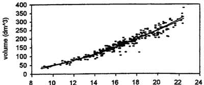
We see that dbh is the only variable that enters squared. That means that dbh has the greatest weight for volume prediction and it means also that, when volume is modeled as a function of dbh, the function must be increasing quadratically. A typical volume function is given in Figure 1.

As with height curves, volume functions are given as mathematical functions that can directly be used in analysis software. In earlier times, volume tables were common, where volume could be read as a function of dbh or in a two way table as a function of dbh and height.

Some more volume function models

Various groups of volume functions are distinguished. The most simple ones are those that model volume as a function exclusively of dbh; these volume models are some times also referred to as volume tariffs. They are applied for smaller area forest inventories like stand inventories. The fact that neither height nor stem shape is explicitly included into that model means that we assume that both height and stem shape can be sufficiently well predicted also by dbh. This is approximately true, above all, for the small area forest inventories, where a major field of application for these volume tariffs exists. Table 1 gives some of these tariffs. It should be observed that, although it is only one subject-matter variable that is being included, it is not simple linear regressions as dbh does also occur as dbh² which is then a second variable in the model.

A further category of volume functions uses dbh and height as independent (predictor) variables. This adds more flexibility to the model to adjust to changing dbh-height relationships as they occur in medium size
forest inventories such as forest enterprise inventories or forest management inventories. This type of volume function assumes that the stem shape can reasonably well be predicted also by dbh. Table 1 gives some of the common models.

Interesting there is the model

\[v=b_1dbh^2h\,\]

where volume is calculated as a function of one single “composed” variable: In fact, this function is identical with the form factor approach to volume calculation, only that here the constant values \(f\) and \(\frac{\pi}{4}\) are together “hidden” in the regression coefficient \(b_1\).

Figure 2 Residual plot of residual volume (\(dm^3\) as Y-axis and dbh (cm) as X-axis showing unequal variance across dbh classes (Kleinn 2007).

Table 1 Different types of models for volume functions, depending on the geographical range of application (after Zöhrer 1980)
\(v=f(dbh)\,\)	\(v={b_0}+{b_1}{dbh}^2\,\)	Also called volume tarifs.
	\(v={b_0}+b_1{dbh}+{b_2}{dbh}^2\,\)	Mainly for local studies where homogeneity of site conditions is expected, including relatively strong relationships between dbh and height and between dbh and form factor.
\(v=f(dbh\mbox{, h}\,)\)	\(v=b_1{dbh}^2h\,\) \(v=v=b_0+b_1{dbh}^2{h}\,\)	Mainly for regional forest inventories.
\(v=f(dbh,h,d_u)\,\)	\(v=b_0+b_1*d_u{dbh}*h\,\)	For larger area forest inventories where heterogeneous site conditions are expected. Therefore, height is included into the model to cope for variability of height curves; and an upper diameter \(d_u\) to cope for variability of form factor.

In large area forest inventories where we can not safely assume that the stem shape is relatively constant or a simple linear function of dbh, it is recommendable to use a further variable that gives information about stem shape, an upper stem diameter. Table 1 gives some of the common models. In the German National Forest Inventory, for example, the diameter at 7 m height is measured at the stem and accordingly processed in volume functions. In fact, not only volume is then derived but the whole taper curve is modeled from the observation of species, dbh and diameter at 7 m.

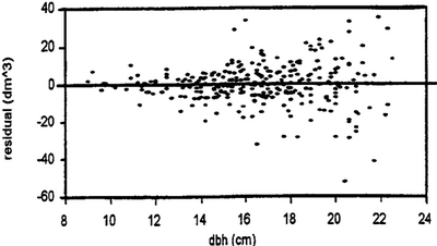
Figure 1 does not only show the typical curvature of a volume function, but also the fact that variability over ''dbh''-classes is not constant over the ''dbh''-range! That means that the assumption of homoscedasticity as stipulated for linear regressions does not hold. This is even clearer illustrated when we graph the residuals over dbh. Residuals are the deviations of the actual values (the volume-dbh data points in Figure 1) from the predicted values (the corresponding values on the regression line). This is shown in Figure 2; it is very obvious that the range (that is, the variability) increases approximately proportional to dbh.

Figure 3 Schematic graphs of confidence intervals for the case of equal variances (left) and the unequal variances case as it presents itself with volume functions (right) (Kleinn 2007).

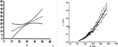
As a consequence of this heteroscedasticity, while we still may safely use the model to predict volume values, we need to take those unequal variances into account when we wish to enter into analysis of variances and errors. That can best be illustrated with the basic example of the confidence intervals to the regression curve; we introduced a regression curve as a curve on which there are mean values for all objects of the population with the same value of the independent variable. Such as for a single mean value we can calculate a confidence interval, we can do the same thing for a regression curve. Just like the mean value changes with \(x\), so does the width of the confidence interval. This is illustrated in Figure 3 on the left hand side for the normal case of equal variances and on the right hand side for the case of unequal variances as it presents itself with volume tariffs. The confidence interval is always symmetrical around the regression curve and for the equal variances case, it is also symmetrical around the overall mean value \(\bar{x},\bar{y}\).

However, for the unequal variance case of volume functions, the confidence interval has the shape of a trumpet. This appears straightforward and logical: the prediction will be best where variability is smallest (at the smaller end of the diameters) and it will be most variable (i.e. wide confidence interval) where the variability is highest (at the larger end of the diameter range); this expectation is clearly represented in the shape of the confidence interval.

However, the confidence intervals for volume functions can not be derived from normal regression analysis. Frequently usual ways out are to use \(log(volume)\) as dependent variable or to use weighted regression.

Volume functions are readily available in many regions for many species. However, it is recommendable not just to use a function that is being offered, but to first make a brief evaluation whether you can trust the model. Part of this evaluation is that you check the related documents and the information given there about the study in which the volume function was generated.

One should certainly not use a volume function (and that holds, in fact, for all statistical models), if the objects of prediction have values of the independent variable which are beyond the range of values of the measurements that had been taken to build the model. If, for example, the sample trees for the volume regression analysis were in a diameter range of 10-50 cm it is not a good idea to use this model for trees beyond 50 cm dbh; that may introduce tremendous errors.

Relevant Questions

The relevant questions that need to be answered in order to be able to know whether a model is reliable or not include:

• How many trees were used to build the model?
• Are the complete statistics given for the model so that the prediction errors can be calculated?
• How was the volume of the sample trees determined? If the volume calculation of the single sample trees is unreliable or inaccurate, the model can not be better!
• What is the range of the independent variables that is covered by a sufficient number of observations? A model shall be used only within the range of values that was used for the model construction.
• How were sample trees selected? If trees were selected according to some criteria, then the volume function is, strictly spoken, valid only for trees that fulfill this criterion.
• From which geographical region did the sample trees come from? If sample trees came from a different region than where the actual study is to be conducted, it can be that the volume function produces wrong results.
• Were outliers eliminated from the analysis; and, if yes, how many?

If there are doubts whether a volume function is suitable for a given purpose, one may opt to calculate the volume of some sample trees and see how the function adjusts to this data. If the fit appears sufficient, then the new data may added to the data base of the old volume function and a new one calculated (that assumes, of course, that the old data are available and accessible).

References

- ↑ 1.0 1.1 Kleinn, C. 2007. Lecture Notes for the Teaching Module Forest Inventory. Department of Forest Inventory and Remote Sensing. Faculty of Forest Science and Forest Ecology, Georg-August-Universität Göttingen. 164 S.
- ↑ Zöhrer F. 1980. Forstinventur – Ein Leitfaden für Studium und Praxis. Verlag Paul Parey. 207 S.