Linear regression
The fundamental concept of regression is to establish a statistical relationship between dependent and independent variables such that predictions of the dependent variable can be done. What we look at here is the linear regression which uses mathematical models in which the coefficients are combined by linear operations. The variables need to be continuous and on a metric scale.
One should be clear that the predicted value is, of course, not the true value of the dependent variable of a particular tree, but it should be interpreted as the mean value of all trees with the same value for the independent variable. That means, the prediction read from a regression is rather an estimation than a measurement! We do illustrate the principle of regression for the simple linear regression, that is for the model
\[y=b_0+b_1x\,\]
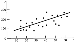
where \(y\) is the dependent variable and \(x\) the independent variable. The graphical representation of this model is a straight line (Figure 1).
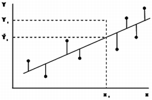
With the statistical technique of regression analysis, the regression coefficients \(b_0\) and \(b_1\) are estimated such that the regression curve (in this case the straight line) fits best to the given data. Of course, a criterion must be defined what the “best” curve and the optimal fit is. In general, the best curve will have some property like that the data points are as close as possible to the regression curve; in regression analysis this is defined as: the best fit is that of the regression curve for which the sum of the squared distances between data points and regression curve is a minimum. This technique is also called the “least squares method”.
The calculations are done in statistics software, but also standard spreadsheet software has this feature even though lesser flexibility than in statistics software.
Requirements
As many other statistical techniques, regression analysis has some assumptions which are particularly relevant if we wish not only to predict data (i.e. read values from the regression curve) but if we wish to do further analysis which also involves analyzing the error of the prediction or the variability of the data points around the regression curve. A typical example of this would be the test whether regression coefficients are significant different from zero. Or the statistical comparison of two regression curves, whether they are statistically significantly different. Application of the least squares technique requires:
- that the data are normally distributed (that is over each class of \(x\) values the \(y\) values shall follow a distribution which is not significantly different from the normal distribution),
- and that the variances of the \(y\) values over all \(x\) classes are equal. Homogeneity of variances is also called homoscedasticity (heteroscedasticity being the contrary when not all variances are equal); and, of course,
- it is also implicitly assumed that the data originate from a random selection process. This is particularly important if we wish to use the regression model as a prediction models for a larger population. Then, the data must come from a random sample. If the regression is only to describe the underlying data set, the assumption of random selection is not relevant.
A regression model is a descriptive statistical model. The relationship established is a statistical relationship in which the regression coefficients estimate to what extent a value of the dependent variable is expected to change when the value of the independent changes.
 Important
- A regression model does not establish or describe a cause-effect relationship. Whether this is there or not is beyond regression analysis. A statistical relationship can also be established for variables which technically have nothing to do with each other (although this would be a somewhat useless exercise).
The more observations we have the more reliable will be the regression model derived from it. An absolute minimum of observations necessary to calculate a regression is defined by the model used. For a straight line we need at least two observations. The optimal number, however, is not easily determined. If there is a strong relationship between the variables, fewer observations are needed in comparison to a situation where there is much variability in the population and not a tight relationship. In forest inventory, as a rule of thumb, we wish to have 20 or more observations for height curves and even more for volume functions.
It is not only the absolute number of observations but also the distribution of the observations over the independent variable which is relevant. The observations should cover the entire range of the independent variable. If the values of the independent variable are clustered in some few and small ranges of the independent variable, then the precision of the regression will be poor.
Example
We may look at regression as a sampling issue: there is a population in which there is a true parametric regression
\[y=\beta_0+\beta_1x\,\]
We wish to know that equation and estimate it from a sample of observations by
\[y=b_0+b_1x\,\]
where \(b_0\) is an estimation for \(\beta_0\) and \(b_1\) is an estimation for \(\beta_1\). The model
\[y=\beta_0+\beta_1x\,\]
is called simple linear model because it has only one independent variable (simple) and the coefficients \(\beta_0\) and \(\beta_1\) are linearly linked (the “+” operation). Other linear models that have more than one independent variable are, for example,
\[y=\beta_0+\beta_1x+\beta_2x^2\,\]
or
\[y=\beta_0+\beta_1x+\beta_2z+\beta_3xz\,\]

