Fixed area plots

Revision as of 07:26, 23 September 2011

General observations

Figure 1 With circular sample plots all trees are taken as sample trees that are within a defined distance (radius) from the sample point, which constitutes the plot center (Kleinn 2007^[1]).

Figure 2 Illustration of the inclusion zone approach: For fixed area circular plots, the inclusion zones are identical for all trees. Those trees are taken as sample trees in whose inclusion zones the sample point comes to lie (Kleinn 2007^[1]).

Figure 3 Typical diameter distribution in a natural forest (Kleinn 2007^[1]).

Figure 4 Nested sub-plots showing 3 circular plots having different sizes, radii, but sharing same plot center (Kleinn 2007^[1]).

Figure 5 Comparison of the inclusion zone approach for nested circular sub-plots (B) and for fixed circular plots (A) (Kleinn 2007^[1]).

Figure 6 Different combination of shapes for nested sub-plots (after Prodan et al. 1997^[2].

Figure 7 A diagram showing an area of reference and projected area into the map plane on a sloping terrain (Kleinn et al 2002^[3]).

Figure 8 Distribution of inclination of forest plots of the second Swiss National Forest Inventory (class 0, 0-9.99%, class 1, 10-19.99%, etc.)(Kleinn et al 2002^[3]).

Figure 9 Mean correction factor for line features as a function of terrain inclination \(\alpha\) (bold line), assuming that the lines have a uniform distribution of angular deviation from the gradient vector. The dashed line gives the standard correction factor cos(\(\alpha\))(Kleinn et al 2002^[3]).

Figure 10 Volume over elevation estimated from the second Swiss National Forest Inventory (Kleinn et al 2002^[3]).

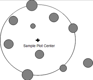
Fixed area sample plots can have various different shapes including circular, square, rectangular and strip. As to which shape is chosen depends on practical and statistical issues. In terms of practical criteria it is mainly the cost which is of interest and which translates into criteria such as terrain conditions and expected frequency of border trees. Border trees cost time because it needs to be carefully checked whether they are in or not and that implies usually additional distance measurements which are not required for the other trees.

From a practical point of view a circular plots is most rapidly installed wherever the visibility in the stand is good. In a tropical forest with dense understory, it is much easier to establish a strip plot where the field crew walks along the central line and measures all trees up to a defined distance to the right and to the left. A circular plot, however, has the lowest expected number of border trees, because, for a given area, the circle is the geometric shape that has the shortest perimeter.

From a practical point of view, coming back to the considerations on spatial autocorrelation, a long rectangular plot (strip plot) covers more different site conditions and is likely to capture more variability per plot. Thus, we may expect higher precision when using strip plots if we compare it with circular plots with the same plot area.

In what refers to the plot size, for a given sampling intensity it is statistically more precise to establish many small plots than few large plots. However, with many small plots, again the cost will be much higher; the decision on Sample size is again a compromise between practical (cost) criteria and statistical (precision). If there is some information on number of stems per hectare, one can calculate, as a rule of thumb, the plot area such that there are on average about 15-20 trees in a sample plot. Typical plot areas are 200 m², 500 m², 1000 m² - but anything is possible.

All trees that have the center of their base inside the plot area are sample trees and are being measured. If a tree is a border tree and it is not obvious whether it is in or out, a measurement must help with that decision. If the tree is exactly on the borderline, then one may count one tree and the next such tree not; but actually, when measuring distances with high accuracy, the case that a tree is exactly on the borderline should be very rare. It is only the center point of the tree base that defines whether a tree is in or out. If center point is in but the tree leans completely outside the plot, this is still an in-tree. If the center is not in the plot, but the entire tree leans into the plot, this tree is not observed.

The inclusion zone concept

We introduced circular fixed area plots such that a sample point is selected and then all trees within a fixed distance (the plot radius r) are taken as sample trees (see Figure 1). While this plot perspective is intuitively clear and understandable, it does not allow to say anything about the per tree inclusion probability. This however, may be an important component of statistical information.

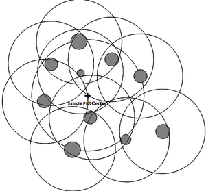
We may change the perspective from the plot perspective to the tree perspective. In that approach, we build a so-called inclusion zone around each tree. The inclusion zone is a measure for the inclusion probability of that particular tree: if a sample point falls into that inclusion zone, then this particular tree is included in a sample. While this sounds maybe complicated, it is extremely helpful in understanding forest inventory sampling and also in deriving unbiased estimators for any plot design.

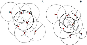
In the case of fixed area circular plots, the inclusion zone that is centered about each tree has the size and shape of the plot, that is circular. All trees, therefore, have the same selection probability. We now imagine the inclusion zones around all trees and select a sample point. Then, all those trees are selected as sample trees for which the sample point falls into their inclusion zone (Figure 2). Of course, at the end, exactly the same trees are selected as with the first approach (of laying out the sample plot), but in this second approach we take the selection probability explicitly into account.

The inclusion zone concept can be applied also to the other plot designs that are being presented in the rest of this chapter.

The plot expansion factor

In forest inventory, we are usually interested in estimates of the total and in estimates per hectare. The immediate per-plot results are not of major interest. In order to get the estimates per hectare one needs to expand the per-plot observation. This is done with a plot expansion factor. For fixed area plots, this expansion factor from the per-plot to the per-hectare estimate is calculated from

\[EF=\frac{1000}{\mbox{PlotSize }(m^2)}\,\].

For example, with a circular fixed area plot of 200 m² or 0.02 ha, the expansion factor is 50. The per-plot observations need to be expanded (multiplied) by \(EF=50\) to produce the per-hectare estimates. This expansion factor is the inverse of the inclusion probability resulting from a certain plot design.

The estimation procedure is illustrated with a simple example: assuming in a 5.0 ha forest stand, 5 plots with 500 m² each are randomly selected. The target variable is the number of stems and we are interested in the estimates per ha and in the estimated total, including the corresponding standard errors. After finishing the inventory, stems per plot observations are 20, 25, 30, 35 and 40 respectively for the 5 plots. It is important to note that each of the plots gives us exactly one independent estimation for the target variable.

The expansion factor is \(EF=20\). Therefore, the per-hectare values expanded from the per-plot values are then 400, 500, 600, 700 and 800, respectively. From these, mean number of stems per ha and its variance can be calculated.

Alternatively, and may be easier, we may calculate all estimations first on a per-plot basis and apply the expansion factor later. For this example, the results per plot are:

Mean number of stems per plot	\(\bar{y}=30\,\)
with variance per plot	\(s^2=62.5\,\)
and standard error	\(s_y=\frac{sw}{\sqrt{n}}=\frac{7.91}{\sqrt{5}}=3.53\,\).

From the standard error, the confidence interval can be calculated where we use for convenience

\[t=2:\mbox{ }ts_y\approx2s_y=2*3.53=7.06\,\],

and therefore:

\[CI=\left[\left(\bar{y}-ts_{\bar{y}}\right)\le\mu\le\left(\bar{y}+ts_{\bar{y}}\right)\right]=\]

\[\left[\left(30-7.06\right)\le\mu\le\left(30+7.06\right)\right]=\left[22.94\le\mu\le37.06\right]\,\]

The results at per-hectare are simply derived by multiplying the per-plot results with the expansion factor, thus for example,

mean number of stems per hectare is	\({\bar{y}}_{ha}=30*20=600\,\)
and standard error is	\(s_{\bar{y}ha}=3.53*20=70.6\mbox{ stems/ha}\,\).

Other estimations follow suit. However, when applying the expansion factor to the variance, it must be observed that the variance comes as squared figure so that the expansion needs to be done with \(EF^2\)! That is, in our example with an estimated per-plot variance of

\[s_{plot}^2=62.5\,\]

the estimated per-hectare variance is

\[s_{ha}^2=s_{plot}^2*EF^2=62.5*20^2=25000\,\].

Cluster plots

So far, we looked at fixed area plots as compact and coherent geometrical shapes like circle and rectangle. However, a sample plot can also come “in pieces”. The most typical examples are the so-called cluster plots (a more detailed description is in the article cluster sampling) which are usually employed in large area forest inventories. Each cluster plot consists of several subunits, called sub-plots, which are located at a certain defined distance apart from each other.

However, we wish to stress yet here that also for cluster plots it holds what was said about randomization and sample size: each randomization step yields one independently selected sample and each one of these such independently selected samples produces exactly one independent observation of the target variable. That means that the entire cluster plot produces one observation of, for example, basal area, and not each sub-plot! This is a frequently committed confusion in forest inventory sampling.

Nested sub-plots

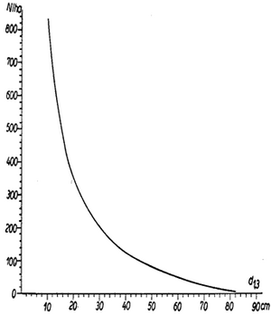
Figure 3 shows a typical diameter distribution in a natural forest, where there is a very high number of small trees and fewer large trees; such a distribution is also called negatively J-shaped. If we lay out a single fixed area plot with a defined radius, our sample plot mirrors what this diameter distribution shows: we will include a high number of small trees and only very few larger trees. Usually, however, we are at least as much interested in the larger trees and do not like to have a very high number of small trees on the plot.

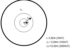
The solution to this is simple: we use nested sub-plots with different sizes as illustrated in Figure 4 for different size classes of trees each; usually, those size classes are diameter classes. Then we can define the plot size for different diameter classes such that in each class (nested sub-plot) there is more or less the target number of sample trees: plots with larger radii are used for larger sample trees and smaller plots for smaller trees.

Nested sub-plots segregate trees by diameter classes and the corresponding plot sizes are different; therefore, analysis must also be made separately for each plot size as there are different plot expansion factors depending on plot size.

The inclusion zone concept can immediately be applied also to nested circular sub-plots as illustrated in Figure 5. There (right hand side), the size of the inclusion zone depend on the diameter of the tree: smaller trees have a smaller inclusion zone and therefore also a smaller selection probability.

Nested sub-plots are not restricted to circular plots but can be applied to any plot shape. Figure 6 gives an illustration of various options. When strip plots are applied, the regeneration plot is frequently taken as a small circular plot of some few square meters. That means that also different plot shapes can be used for the differently sized plots.

Slope correction

Results from forest inventories are area-related; examples are volume/ha, basal area/ha, number of stems/ha. The area to which these measures refer is the map area; that is the horizontal projection of the terrain into the map plane. If we lay out a circular plot with a defined radius on the slope, the projected area in the map plane will be different. This is obviously not desired but if we wish to make an extrapolation of the per-plot observation to the per hectare observation, then all related areas must refer to the same reference system, and that is the map plane.

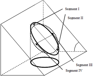
As a consequence, if we have a defined plot area that is to be used for all sample plots, this area is defined in the map plane. If plots are to be laid out in sloped terrain, the plot area on the slope must be larger such that the target plot area results when the plot is horizontally projected. This is illustrated for circular fixed area plots in Figure 7.

If we define (Figure 7) the target plot area in the map plane, then this plot becomes an ellipse when projected in the oblique plane, and this ellipse has a larger area than the original plot in the map plane. If electronic range finders that can also measure slope angle are used for distance measurement, then this ellipse can easily be laid out in the field where the two radii of the ellipse are automatically calculated. If \(r\) is the radius of the original plot in the map plane and \(\alpha\) the slope angle, then the two radii of the ellipse are \(r\) and

\[\frac{r}{\mbox{cos }\alpha}.\,\]

If we do not have the possibility of making automatic correction, another way of slope correction must be applied. The idea is to find the radius of the circle that has an area equal to the one of the ellipse. By that, we guarantee that the plot has the target area when projected into the map plane; by this procedure, we accept that the plot as projected into the map plane has an ellipse shape.

Let´s assume that the circular sample plot has the defined area (in the plane)

\[F_p={\pi}r^2.\,\]

If projected to a slope with slope angle \(\alpha\), an ellipse results with radii \(r\) and

\[\frac{r}{\mbox{cos }\alpha}\,\]

which has the area (on the slope),

\[F_{slope}=\pi r\frac{r}{\mbox{cos }\alpha}=\frac{\pi r^2}{\mbox{cos }\alpha}.\,\]

This is larger than the one in the map plane. We wish now to find the radius \(r_{slope}\) of the circle that has that area and we find it as

\[r_{slope}=\frac{r}{\sqrt{\mbox{cos }\alpha}}.\,\]

That means: in sloped terrain, the original plot radius needs to be multiplied by the slope correction factor

\[\frac{1}{\sqrt{\mbox{cos }\alpha}}.\,\]

By that, a larger circle is generated which has an area equal to the area to the ellipse that would result if we projected the original plot size into the map plane. The correction factor is obviously always larger than 1.

For application in forest inventories, slope correction factors are usually pre-calculated and tabulated. Alternatively, it is programmed in the field computers.

The slope correction is commonly applied for slopes larger than 10%. For smaller slopes the deviation is so small that it is accepted without correction.

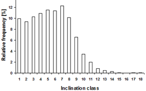
Slope correction is in particular relevant, when inventorying forests in hilly and mountainous regions. Figure 8 illustrates that for the National Forest Inventory of Switzerland. There, only about 10% of the sample plots are in terrain with slopes less than 10%, and a considerable percentage (around 5%) are even on slopes with more than 100% inclination!

Slope correction for line features

In some inventories, also linear features are measured, like length of roads; length of water (creeks); and length of forest boundary. In principle, we can proceed like with all other variables: observing what we find on the plot and use the expansion factor to extrapolate to the whole of the inventory region (or to a per-hectare-estimate). However, in sloped terrain, the correct correction procedure must obviously be different from the described general slope correction, because the actual projected length of a line feature at the slope is a function of the actual slope of the line itself which is not the overall slope of the terrain!

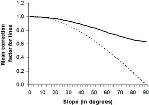
The projection of an individual line segment must be based on its actual inclination. Application of any gross correction factor to all sampled line segments would not be correct. However, if no information on the orientation of the individual line segments is available; one may want to employ a mean correction factor, if we assume that the lines are uniformly distributed over all possible directions.

The correction line in Figure 9 was derived numerically, it is approximated by

\[\mbox{cos}^2\frac{\alpha}{2.1}.\,\]

It assumes uniform angular distribution of the orientation of line segments relative to the slope gradient. It gives good results for the range of slopes that matter for forest inventories, where the deviation from the numerically derived values is less than 1% for inclinations

\[0\le\alpha\le60°.\,\]

Effects of slope correction

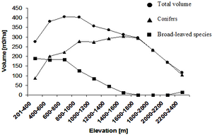
Concern is some time expressed that the usual slope correction ‑ that, while maintaining the target plot area, changes the shape of the plot from the correct ellipse to a larger circle ‑ introduces a systematic error in particular in cases where the target variable has a gradient along the slope gradient; then, more “average” elements will be observed (in segment III and IV of Figure 7) in the size-adjusted circle in the field, and lesser observations are made along the gradient (that is, in segments I and II). In fact, there are variables that change with altitude, i.e. have a gradient along the slope. Figure 10 illustrates that for volume per hectare as a result from the Swiss National Forest Inventory (here, it is interesting to note the difference between coniferous and broadleaved species). Although the gradient is significant, however, it is too small to be relevant in the context of the slope correction. For volume/ha, at least, we do not expect the slope correction to cause problems.

Example: Slope correction with fixed area plots

Suppose, we measure a 1000 m² fixed area plot on a slope of 30% and we count 10 trees in that plot. Without correcting for slope, we calculate an expansion factor of 10 and the estimation is 100 trees per hectare.

However, the 1000 m² plot on the slope (r=17.84m) becomes an ellipse when projected to the map plane with the two radii \(r_1=17.84m\) and \(r_2=17.088m=r_1*\mbox{cos }\alpha\) and an area of

\[F_E={\pi}r_1r_2=957.8m^2=1000m^2*\mbox{cos }\alpha.\,\]

Where, the factor of 10 is valid for all plots on slopes less than 10%, the correct expansion factor for the 1000 m² circle at 30% has to be larger, as the circle becomes a smaller ellipse when projected to the map plane. The calculation is as follows:

\[\frac{10000m^2}{1000m^2}*\mbox{cos }\alpha=\frac{10000}{957.8}=10.44,\,\]

and the correct estimation for the number of trees per hectare is:

\[104.4=100*\frac{1}{\mbox{cos }\alpha}.\,\]

References

1. ↑ ^{1.0 1.1 1.2 1.3 1.4} Kleinn, C. 2007. Lecture Notes for the Teaching Module Forest Inventory. Department of Forest Inventory and Remote Sensing. Faculty of Forest Science and Forest Ecology, Georg-August-Universität Göttingen. 164 S.
2. ↑ Prodan M., R. Peters, F. Cox and P. Real 1997. Mensura forestal. Serie investigación y educación en desarrollo sostenible. IICA/GTZ. 561p.
3. ↑ ^{3.0 3.1 3.2 3.3} Kleinn C., B. Traub and C. Hoffmann 2002. A note on the slope correction and the estimation of the length of line features. Canadian Journal of Forest Research 32(4):751-756.