Resource assessment exercises: fixed area plots
| Line 115: | Line 115: | ||
== References == | == References == | ||
| − | < | + | <references/> |
[[category:Response designs in resource assessment (2014)|Fixed area plots]] | [[category:Response designs in resource assessment (2014)|Fixed area plots]] | ||
Revision as of 19:14, 8 July 2014
| sorry: |
This section is still under construction! This article was last modified on 07/8/2014. If you have comments please use the Discussion page or contribute to the article! |
Suppose a forest inventory has been conducted in the simulated 50 hectare forest. In total \(n=50\) fixed area sample plots with a radius of \(r=15.45\) meters have been randomly placed in the forest (see Figure A). The area covered by a single plot is 0.08 hectares. If parts of the plot lied outside the forest area, this part has been mirrored back (see Kleinn (2013)[1] and the this article for details). For all trees with a DBH \(\geq\) 5 cm the DBH (cm), height (m) and tree species has been recorded. Furthermore the azimuth (1–360\(^\circ\)) and distance (m) of each tree to the plot center on which the tree was found has been measured.
The “forest inventory” was conducted in . The resulting dataset (as well as all other data we need in subsequent sections) is stored in the file MES.RData. We load the data into the workspace.
## 'data.frame':    2158 obs. of  9 variables:
##  $ plotID  : num  1 1 1 1 1 1 1 1 1 1 ...
##  $ plot.x  : num  620753 620753 620753 620753 620753 ...
##  $ plot.y  : num  5886461 5886461 5886461 5886461 5886461 ...
##  $ species : num  1 1 1 1 1 1 1 1 1 1 ...
##  $ dbh     : num  21 23 26 26 21 13 25 22 26 21 ...
##  $ height  : num  11.86 12.06 11.08 10.36 9.36 ...
##  $ ab      : num  0.1056 0.1292 0.152 0.1421 0.0831 ...
##  $ azimuth : num  101.1 235.7 63.3 309.4 280 ...
##  $ distance: num  12.22 12.75 8.05 9.52 13.98 ...
The variable plotID indicates on which plot the tree was found. How many trees are there on each of the 50 plots?
##
##  1  2  3  4  5  6  7  8  9 10 11 12 13 14 15 16 17 18 19 20 21 22 23 24 25 26
## 47 63 92 46 42 66 52 66 49 74 79 52 48 40 30 56 67 51 59 60 45 44 49 76 35 33
## 27 28 29 30 31 32 33 34 35 36 37 38 39 40 41 42 43 44 45 46 47 48 49 50
## 25 37 29 36 31 39 54 20 24 27 21 25 38 32 37 31 39 16 20 36 29 33 21 37
Suppose we would like to estimate the number of stems ha\(^{-1}\) in the forest. Since each plot covers an area of 0.08 hectares we need to compute the so-called plot expansion factor in order to be able to estimate the stems per hectare. If we have a radius of \(r=15.45\) the area covered by one plot is 750 m\(^2\).
## [1] 13.33
When we multiply the number of trees of each plot with the expansion factor we obtain the number of trees per hectare and plot.
##
##      1      2      3      4      5      6      7      8      9     10
##  626.7  840.0 1226.7  613.3  560.0  880.0  693.3  880.0  653.3  986.7
The mean of stems.ha.i provides a population estimate of the stems per hectare.
## [1] 575.5
How good is our estimate (see Subsection [sub:se])?
## [1] 50
## [1] 32.43
# relative SE in %
## [1] 5.636
## [1] 510.3
## [1] 640.6
We know the truth.
## [1] 600
Next, we estimate the BA ha\(^{-1}\). Firstly, we need to calculate the BA (m\(^2\)) for each tree. Secondly, the total BA is calculated for each plot. Thirdly, the results are multiplied with the expansion factor. Finally, the BA ha\(^{-1}\) is estimated for the forest.
## [1] 33.17
We estimate the relative standard error in percent:
## [1] 10.29
Thus, we expect the BA ha\(^{-1}\) to be 33.17 \(\pm\) 6.86 m\(^2\). The parametric BA ha\(^{-1}\) is,
## [1] 28.66
Finally, we estimate the proportion of beech trees in the forest.
## [1] 0.6429
There is one plot (plotID 5) without any beech tree. One way to solve the problem would be use the levels argument of the factor() function.
## [1] 0.6429
The estimated standard error is
## [1] 0.06845
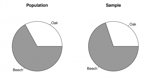
Figure [fig:pie] shows to pie charts of the proportion of beech trees in the population (left) and the sample (right).
[fig:pie]
Exercises
- Load the file
exercises.RDatainto the workspace. The file contains adata.framenamedfixed.area.Exthat holds data from a forest inventory using fixed area sample plots. The size of the plot is 750 m\(^2\). - Calculate the expansion factor for a plot.
- How large is \(n\) (
plotIDgives the plot number for each tree)? - Estimate the BA ha\(^{-1}\) and the number of stems per hectare. Provide an estimate of the standard error and construct confidence intervals for \(\alpha=0.10\).
Related articles
References
- ↑ Kleinn, C., 2013. Lecture Notes for the Teaching Module Forest Inventory.
