Resource assessment exercises: fixed area plots

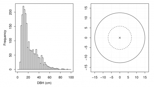
Suppose a forest inventory has been conducted in the simulated 50 hectare forest. In total \(n=50\) fixed area sample plots with a radius of \(r=15.45\) meters have been randomly placed in the forest (see Figure A). The area covered by a single plot is 0.08 hectares. If parts of the plot lay outside the forest area, this part was mirrored back (see Kleinn (2013) and this article for details). For all trees with a DBH \(\geq\) 5 cm the DBH (cm), height (m) and tree species was recorded. Furthermore the azimuth (1–360\(^\circ\)) and distance (m) of each tree to the plot center on which the tree was found was measured.

Figure A: Histogram of DBH in fixed.area and nested sample plot

The “forest inventory” was conducted in R. The resulting dataset (as well as all other data we need in subsequent sections) is stored in the file MES.RData. We load the data into the R workspace.

load("./data/MES.RData") # Don't forget to adjust the path!
str(fixed.area) # Data for the fixed area plots

## 'data.frame':    2158 obs. of  9 variables:
##  $ plotID  : num  1 1 1 1 1 1 1 1 1 1 ...
##  $ plot.x  : num  620753 620753 620753 620753 620753 ...
##  $ plot.y  : num  5886461 5886461 5886461 5886461 5886461 ...
##  $ species : num  1 1 1 1 1 1 1 1 1 1 ...
##  $ dbh     : num  21 23 26 26 21 13 25 22 26 21 ...
##  $ height  : num  11.86 12.06 11.08 10.36 9.36 ...
##  $ ab      : num  0.1056 0.1292 0.152 0.1421 0.0831 ...
##  $ azimuth : num  101.1 235.7 63.3 309.4 280 ...
##  $ distance: num  12.22 12.75 8.05 9.52 13.98 ...

The variable plotID indicates on which plot the tree was found. How many trees are there on each of the 50 plots?

n.trees <- table(fixed.area$plotID)
n.trees

## 
##  1  2  3  4  5  6  7  8  9 10 11 12 13 14 15 16 17 18 19 20 21 22 23 24 25 26 
## 47 63 92 46 42 66 52 66 49 74 79 52 48 40 30 56 67 51 59 60 45 44 49 76 35 33 
## 27 28 29 30 31 32 33 34 35 36 37 38 39 40 41 42 43 44 45 46 47 48 49 50 
## 25 37 29 36 31 39 54 20 24 27 21 25 38 32 37 31 39 16 20 36 29 33 21 37

What the function table() does

The function table(x) provides the counts of unique values in a vector. E.g., table(fixed.area$stratum) would give us the number of trees sampled in each stratum.

Suppose we would like to estimate the number of stems ha\(^{-1}\) in the forest. Since each plot covers an area of 0.08 hectares we need to compute the so-called plot expansion factor in order to be able to estimate the stems per hectare. If we have a radius of \(r=15.45\) the area covered by one plot is 750 m\(^2\).

expf <- 10000/750 # expansion factor for a plot of 750 square meters
expf

## [1] 13.33

When we multiply the number of trees of each plot with the expansion factor we obtain the number of trees per hectare and plot.

stems.ha.i <- n.trees * expf 
stems.ha.i[1:10] # to save space, only the first 10 plots are printed

## 
##      1      2      3      4      5      6      7      8      9     10 
##  626.7  840.0 1226.7  613.3  560.0  880.0  693.3  880.0  653.3  986.7

Indexing using squared brackets []

To access individual entries (or ranges of entries) in a vector we can use squared brackets. E.g. trees$dbh[2] selects the second value of dbh in trees. Instead of explicitly naming variables using the dollar sign, e.g., trees$dbh, we can also use the squared brackets. The principle is as follows: data.object[row(s), column(s)]. E.g., trees[c(1, 4:10), c(1,3)] would print out the first, fourth to tenth row, and the first and third column of trees.

The mean of stems.ha.i provides a population estimate of the stems per hectare.

mean(stems.ha.i) 

## [1] 575.5

How good is our estimate (see standard error and confidence intervals)?

(n <- length(unique(fixed.area$plotID))) # sample size

## [1] 50

(se <- sd(stems.ha.i)/sqrt(n)) # estimated standard error (SE)

## [1] 32.43

(relse <- se/mean(stems.ha.i) * 100) # relative SE in %

## [1] 5.636

mean(stems.ha.i) - se * qt(0.975, n - 1) # lower confidence limit

## [1] 510.3

mean(stems.ha.i) + se * qt(0,975, n - 1) # upper confidence limit

## [1] 640.6

What the function unique() does

The function unique(x) reports the unique values in x. E.g., for a vector $1,2,2,3,3,3$, unique(c(1,2,2,3,3,3)) would print 1, 2, 3, the length would be three.

We know the truth.

stems.ha <- nrow(trees)/50
stems.ha

## [1] 600

Next, we estimate the BA ha\(^{-1}\). First, we need to calculate the BA (m\(^2\)) for each tree. Second, the total BA is calculated for each plot. Third, the results are multiplied with the expansion factor. Finally, the BA ha\(^{-1}\) is estimated for the forest.

fixed.area$ba <- ((fixed.area$dbh/2)^2 * pi)/10000
sum.ba <- tapply(fixed.area$ba, fixed.area$plotID, sum)
ba.ha <- sum.ba * expf
(ba.fixed.area.mean <- mean(ba.ha))

## [1] 33.17

We estimate the relative standard error in percent:

(ba.fixed.area.ser <- sd(ba.ha)/sqrt(n)/mean(ba.ha) * 100)

## [1] 10.29

Thus, we expect the BA ha\(^{-1}\) to be 33.17 \(\pm\) 6.86 m\(^2\). The parametric BA ha\(^{-1}\) is,

sum(trees[, "ba"])/50

## [1] 28.66

Finally, we estimate the proportion of beech trees in the forest.

fixed.area.beech <- fixed.area[fixed.area$species == 2, ]
n.beech.plot <- table(fixed.area.beech$plotID)
mean(n.beech.plot/n.trees)

## [1] 0.6429

There is one plot (plotID 5) without any beech tree. One way to solve the problem would be to use the levels argument of the factor() function.

n.beech.plot <- table(factor(fixed.area.beech$plotID, levels = 1:50))
(p <- mean(n.beech.plot/n.trees))

## [1] 0.6429

What the function factor() does

The function factor(x) is used to encode a vector into factor levels. The levels argument is used to specify the factor levels.

The estimated standard error is

q <- 1 - p
sqrt((p * q)/(n - 1))

## [1] 0.06845

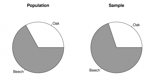
Figure B shows two pie charts of the proportion of beech trees in the population (left) and the sample (right). You can recreate the plots with the following code:

pie(table(trees$species), labels = c("Oak", "Beech"), main = "Population")
pie(table(fixed.area$species), labels = c("Oak", "Beech"), main = "Sample")

Figure B: Pie chart of the species shares in the population (left) and in the sample (right).

Additional Exercises

• Load the file exercises.RData into the R workspace. The file contains a data.frame named fixed.area.Ex that holds data from a forest inventory using fixed area sample plots. The size of the plot is 750 m\(^2\).
• Calculate the expansion factor for a plot.
• How large is \(n\) (plotID gives the plot number for each tree)?
• Estimate the BA ha\(^{-1}\) and the number of stems per hectare. Provide an estimate of the standard error and construct confidence intervals for \(\alpha=0.10\).

Related articles

• Previous article: introduction to response designs
• Next article: nested fixed area plots
• Fixed area plots at the stand boundary

References

- ↑ Kleinn, C., 2013. Lecture Notes for the Teaching Module Forest Inventory.