Height curve

Revision as of 16:22, 26 October 2013

General observations

Figure 1 Height curves in even aged stands exhibit typical changes over time which are depicted here simplified and schematically: they get flatter, shift right on the dbh axis and up on the height axis and cover a wider range of diameters (“become longer”).

Figure 2 Simple linear regression with ln(dbh) as sole independent variable. In addition to the data points, the mean heights per 10cm dbh-class are given. In this case, the model is obviously not flexible enough to adjust well to the height values for very large diameters.

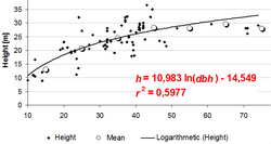
The relationship between height and dbh, where it needs to be defined first which height is meant; standard height curves refer to total tree height. While regression is the standard to determine a height curve, there are other techniques which are less statistically rigorous. A visual (or manual) fit can be done when the dbh/height points are drawn in a grid system. From that drawn curve, height values can directly be read without the requirement to define a mathematical model and to calculate its coefficients. For a so-called half-graphical fitting, in a first step, mean height values are calculated for diameter classes (the width of these classes needs to be determined); the manual fit is then done for the set of mean values and not for all measurement points; by that, the fit can graphically easier be done (which is illustrated in Figure 2).

Height curves are nowadays usually given as mathematical functions that can be integrated into analysis software. In former times, they were given in tabular form so that for each diameter (or diameter class) the height could be read directly.

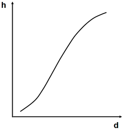
The shape of the height curve as given in Figure 2 is typical for even-aged stands. The curve is steeper in the range of smaller diameters and flattens for larger diameters. It may even be that the curve goes down a little bit for very large trees; this can be the case in regions with site differences where the very large trees on poorer sites are less tall then slightly smaller trees on better sites.

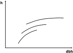
It must be clearly understood that the height curve describes the status of the relationship between dbh and height for a given point in time. It is not a growth curve. It can, therefore, not be used to predict the height of a particular tree for later points in time! How height curves in even-aged stands do commonly change over time is depicted in Figure 1.

Modeling height curves

Figure 3 The same height curve as in Figure 2 but drawn in a grid with ln(dbh) on the abscissa instead of dbh only.

Figure 4 A typical height curve in a natural uneven-aged stand. If the forest is in a “steady state”, This curve does not change over time and can simultaneously be interpreted as growth curve (from Prodan et al. 1997^[1].)

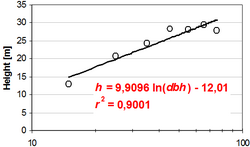
There are many different models that have been used to fit height curves, some of them are given in Table 1. The simple quadratic model (model (1) in Table 1) is well suited in most cases. Model (2) in Table 1 is interesting because it is a simple linear model with only one independent variable, the logarithm of dbh; this model produces a straight line when drawn in a half-logarithmic grid but produces a curve well suited for height curves when drawn in normal linear grids (compare Figure 2 and Figure 3).

In natural forests, where all age classes are present on the same area, the height curve has a different shape, see Figure 4. If the forest is in a balanced steady state, shape and position of the height curve remains the same. In this case, for natural forests, the height curve corresponds to the height growth curve and may be accordingly interpreted.

Height curves are usually developed per species or per species group. They are readily available in many regions where intensive forest management is practiced. But it may be that new height curves need to be generated as part of an inventory project. Then, dbh and height need to be carefully measured on a number of stems (as many as feasible), the model defined and the coefficients calculated. This is frequently integrated into the inventory work as follows: dbh is measured for all sample trees, but height only for a small sub-set, for example on each sample plot the one or two trees closest to the plot center are height measured. From these dbh/height pairs of values the height curve is calculated which allows then to predict the height also for all other trees where no height measurement has been taken.

References

1. ↑ Prodan M., R. Peters, F. Cox and P. Real. 1997.Mensura forestal. Serie investigación y educación en desarrollo sostenible. IICA/GTZ. 561p.