Horvitz-Thompson estimator
| Line 27: | Line 27: | ||
:<math>v\hat ar(\hat \tau) = \frac {N - \nu}{N} \frac {1}{\nu} \frac {\sum_{i=1}^\nu (\tau_i -\hat \tau)^2}{\nu - 1}</math> | :<math>v\hat ar(\hat \tau) = \frac {N - \nu}{N} \frac {1}{\nu} \frac {\sum_{i=1}^\nu (\tau_i -\hat \tau)^2}{\nu - 1}</math> | ||
| − | where | + | where <math>\tau_i</math> is the estimation for the total that results from each of the <math>\nu</math> sample. |
| − | + | ||
| − | + | ||
Latest revision as of 13:22, 26 October 2013
Assuming that with any design, with or without replacement, the probability of including unit i in the sample is \(\pi_i\) (>0), for i=1,2,…, N. The inclusion probability \(\pi_i\) can be calculated from the selection probability \(p_i\) and the corresponding complementary probability (1-pi), which is the probability that the element is not included into the sample at a particular draw.
After n sample draws, the probability that element i is eventually included into the sample is \(\pi\)=1 - (1-pi)n, where (1 - pi)n is the probability that the particular element is not included after n draws; the complementary probability to this is then the probability that the element is eventually in the sample (at least selected once).
The Horvitz-Thompson estimator can be applied for sampling with or without replacement, but here it is illustrated for the case with replacement.
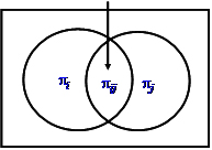
For the variance calculation with the Horvitz-Thompson estimator we also need to know the joint inclusion probability \(\pi_{ij}\) of two elements i and j after n sample draws, that is the probability that both i and j are eventually in the sample, after n draws. This joint inclusion probability is calculated from the two selection probabilities and the two inclusion probabilities after \(\pi_{ij} = \pi_i + \pi_j - \{ 1 - (1 - p_i - p_j)^n \} \) and can be illustrated as in Figure 1.
The Horvitz-Thompson estimator for the total is \(\hat \tau = \sum_{i=1}^\nu \frac {y_i}{\pi_i}\)
where the sum goes over the \(\nu\) distinct elements (where \(\nu\) is the Greek letter nu) in the sample of size n (and not over all n elements)
The parametric error variance of the total is
\[var(\hat \tau)=\sum_{i=1}^\nu \left (\frac {1 - \pi_i}{\pi_i} \right ) y_i^2 + \sum_{i=1}^N \sum_{j \ne i} \left (\frac {\pi_{ij} - \pi_i \pi_j}{\pi_i \pi_j} \right ) y_i y_j\]
which is estimated by
\[v\hat ar(\hat \tau)=\sum_{i=1}^\nu \left (\frac {1 - \pi_i}{\pi_i^2} \right ) y_i^2 + \sum_{i=1}^N \sum_{j \ne i} \left (\frac {\pi_{ij} - \pi_i \pi_j}{\pi_i \pi_j} \right ) \frac {y_i y_j}{\pi_{ij}}\]
A simpler (but slightly biased) approximation for the estimated error variance of the total is
\[v\hat ar(\hat \tau) = \frac {N - \nu}{N} \frac {1}{\nu} \frac {\sum_{i=1}^\nu (\tau_i -\hat \tau)^2}{\nu - 1}\]
where \(\tau_i\) is the estimation for the total that results from each of the \(\nu\) sample.
 Horvitz-Thompson estimator example: application example
