Individual Tree Detection (ITC)

Filter the CHM derived from LiDAR data

We use a Canopy Height Model (CHM) derived from LiDAR data as decribed here to detect Individual Tree Crowns (ITC). Two preprocessing steps prepare a watershed segmentation approach: (1) Gaussian filtering and (2) inversion of a CHM.

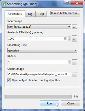
• In the search engine of the Processing Toolbox, type smooth and select Smoothing (gaussian) under Image filtering of the Orfeo Toolbox.
• Select the CHM raster data file in GeoTiff format as input layer.
• The smoothing type is gaussian.
• The circular structuring element has a radius of 2 pixels.
• Enter name and path for an output file.
• Click on Run.

Invert the CHM

Now the smoothed CHM will be inverted.

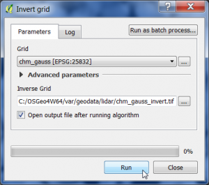
• In the search engine of the Processing Toolbox, type invert and select Invert grid under Raster tools of SAGA.
• Select the smoothed CHM raster data file from previous step as input layer.
• Enter name and path for an output file.
• Click on Run.

Watershed segmentation

• In the search engine of the Processing Toolbox, type watershed and select Watershed segmentation under Image Analysis of SAGA.
• Select the inverted and smoothed CHM raster data file as input Grid.
• The Output is Segment ID
• Select as Method the flow accumulation of Minima
• Seed points: enter name and path for a vector point output file.
• Click on Run.

Extracting tree heights

We extract normalized heights from the original CHM using the QGIS point sampling plugin.

1. Click Plugins --> Manage and Install Plugins.
2. Type in the search bar Point sampling tool, click on the plugin name and then on Install plugin.
3. Load the single band raster file chm.tif.
4. Load the vector point file Seed points.shp'.
5. Make sure that both layers are ticked in the TOC.
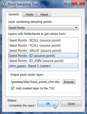
6. Open the Point Sampling Tool clicking .
7. Specify the output of the resulting vector file marking column with CTRL + left click.
8. Enter an output shapefile name seed_points_chm.shp and path by clicking Browse.
9. Confirm with OK. The new layer is added to the Layer Panel .

• Right click on the layer name in the TOC and open the Attribute table of the new vector layer.
• Toggle editing on.
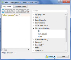
• Select features using an expression.
• Type in the expression editor: "chm" <= 3 and click Select. All points with heights below 3m are now selected.
• Click Delete selected features.
• Toggle editing off.

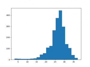
We produce a histogram of the tree height distribution in the forest stand.

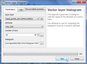
• In the search engine of the Processing Toolbox, type histogram and select Vector layer histogram under Graphics of QGIS geoalgorithms.
• Select the shapefile name seed_points_chm.shp as input layer.
• Select as Attribute the column with the extracted height values chm.
• Select the number of histogram bins: 20.
• Enter name and path for a graphic output file.
• Click on Run.

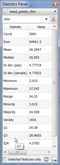
You want to produce a statistical summary of tree heights in the stand? Use the QGIS Statistics Panel:

• Open View --> Statistical summary to open the Statistics Panel.
• The layer seed_points_chm.shp need to be loaded in the TOC.
• Choose seed_points_chm in the top combo box, then choose chm in the field selector box of the Statistics Panel.
• The statistical summary for tree heights of the forest stand is displayed in the Statistics Panel.

Report on the mean stand height. What means Q3?

Graphical Processing Tool Model

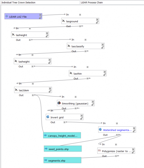
Exhausting to follow all these work steps? You can use a prepared graphical processing toolbox model in the lidar tutorial data set: ITC_detection.model.

1. Open QGIS and go to the Processing Toolbox; if the Toolbox is not opened go to Processing --> Toolbox to activate it. Once the Toolbox is opened go to Models --> Tools --> Add model from file and load the previously downloaded model.
2. The model should appear in the Models tab. Double click on it to execute.
3. A window showing the different input and outputs should appear, just as if you were using any other geoalgorithm of the Processing Toolbox.
4. You will just need to provide the model with the LiDAR data input file in LAZ format.