Statistical estimations
| Line 52: | Line 52: | ||
==Point estimates vs. interval estimates== | ==Point estimates vs. interval estimates== | ||
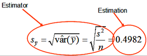
| − | For each statistic that is been estimated (such as a mean, a variance, a correlation coefficient, …) there are two basic types of statistical estimations, the “point estimate”, which estimates the parameter of interest, and the “interval estimate” which estimates the precision of the point estimate. | + | For each statistic that is been estimated (such as a mean, a variance, a correlation coefficient, …) there are two basic types of statistical estimations, the “point estimate”, which estimates the parameter of interest, and the “interval estimate” which estimates the precision of the point estimate. The [[standard error]] is a measure of the variability of estimation. |
| − | + | ||
| − | + | ||
| − | The standard error is a measure of the variability of estimation | + | |
| − | + | ||
| − | + | ||
| − | + | ||
| − | + | ||
| − | + | ||
| − | + | ||
| − | + | ||
| − | + | ||
| − | + | ||
| − | + | ||
==Confidence Interval (CI)== | ==Confidence Interval (CI)== | ||
Revision as of 18:32, 27 October 2013

We are interested to know the true population parameters but are not able to determine them. We use, therefore, sampling to produce estimations which we take then as approximations for the true population values; always knowing that estimations carry an error.
Estimations are the principal result of sampling studies. All results of a sample are estimations and must be interpreted as such; they help us to learn something about the unknown parameters of the population of interest.
Contents |
Notations
There are some conventions in what refers to the notation of population parameters and estimated statistics:
| parametric mean | \(\mu\,\) |
| estimated mean | \(\bar{y}\,\) |
| parametric variance | \(\sigma^2\,\) |
| estimated variance | \(s^2\,\) |
| regression coefficients | \(\beta\,\) |
| estimated coefficients | \(b\,\) |
| unknown population parameter | \(\theta\,\) |
| sample based estimation | \(\hat\theta\,\) |
The “ ^ ” is generally used to make clear that an expression is a sample based estimation. If, for example the variance of variable \(X\) is denoted \(var(X)\), then the estimated variance of \(X\) would be written as \(\hat{var}(X)\). For the estimated mean and the estimated variance, one could also write \(\hat\mu\) and \(\hat\sigma^2\), respectively.
There are various important desirable characteristics of estimators, among them unbiasedness and relative efficiency (when comparing to other estimators); these two are briefly characterized in what follows. It is emphasized here that these are properties of the estimators, not of the estimations!
Relative efficiency
If, in a sampling study, we have the choice between different sampling designs or within the same sampling design between different estimators, we wish to apply the most efficient one; that is the one that yields best precision for a given effort. This involves the comparison with alternative estimators or/and other sampling designs:
If \(\hat\theta_1\) and \(\hat\theta_2\) are two unbiased estimators, relative efficiency is simply calculated as the ratio of the error variances of the two estimators.
\[RE=\frac{V(\hat\theta_1)}{V(\hat\theta_2)}\]
It should be observed that this is valid for \(var(\hat\theta)\) and not necessarily for \(\hat {var}(\hat\theta)\); that is, from data of a sampling study we can only estimate the relative efficiency.
Point estimates vs. interval estimates
For each statistic that is been estimated (such as a mean, a variance, a correlation coefficient, …) there are two basic types of statistical estimations, the “point estimate”, which estimates the parameter of interest, and the “interval estimate” which estimates the precision of the point estimate. The standard error is a measure of the variability of estimation.
Confidence Interval (CI)
For an estimation, the confidence interval defines an upper and lower limit within which the true (population) value is expected to come to lie with a defined probability. This probability is frequently set to 95%, meaning that an error of is accepted (other a are also possible, of course). In order to be able to build such a confidence interval, the distribution of the estimated values need to be known. It is known in sampling statistics, that the estimated mean follows a normal distribution if the sample is large (n>>30, say), and the t distribution with ν degrees of freedom when the sample is small (n<30, say). For a defined value α for the error probability the width of the confidence interval for the estimated mean is given by , where t comes from the t-distribution and depends on sample size (df = degrees of freedom=n-1) and the error probability. Then,
As with the standard error of the mean, the width of the confidence interval (CI) can be given in absolute (in units of the mean value) or in relative terms (in %, relative to the estimated mean).
If an estimation is accompanied by a precision statement, one must clearly say whether that is the standard error or half the width of the confidence interval! For larger sample sizes and α=5%, the t-value is , that is around 2 so that as a rule of thumb we may say that half the width of the confidence interval is given by twice the standard error: . For smaller sample sizes, the t-value will be larger.
References
- ↑ Kleinn, C. 2007. Lecture Notes for the Teaching Module Forest Inventory. Department of Forest Inventory and Remote Sensing. Faculty of Forest Science and Forest Ecology, Georg-August-Universität Göttingen. 164 S.