File list
This special page shows all uploaded files. When filtered by user, only files where that user uploaded the most recent version of the file are shown.
| Date | Thumbnail | Size | User | Description | Versions | |
|---|---|---|---|---|---|---|
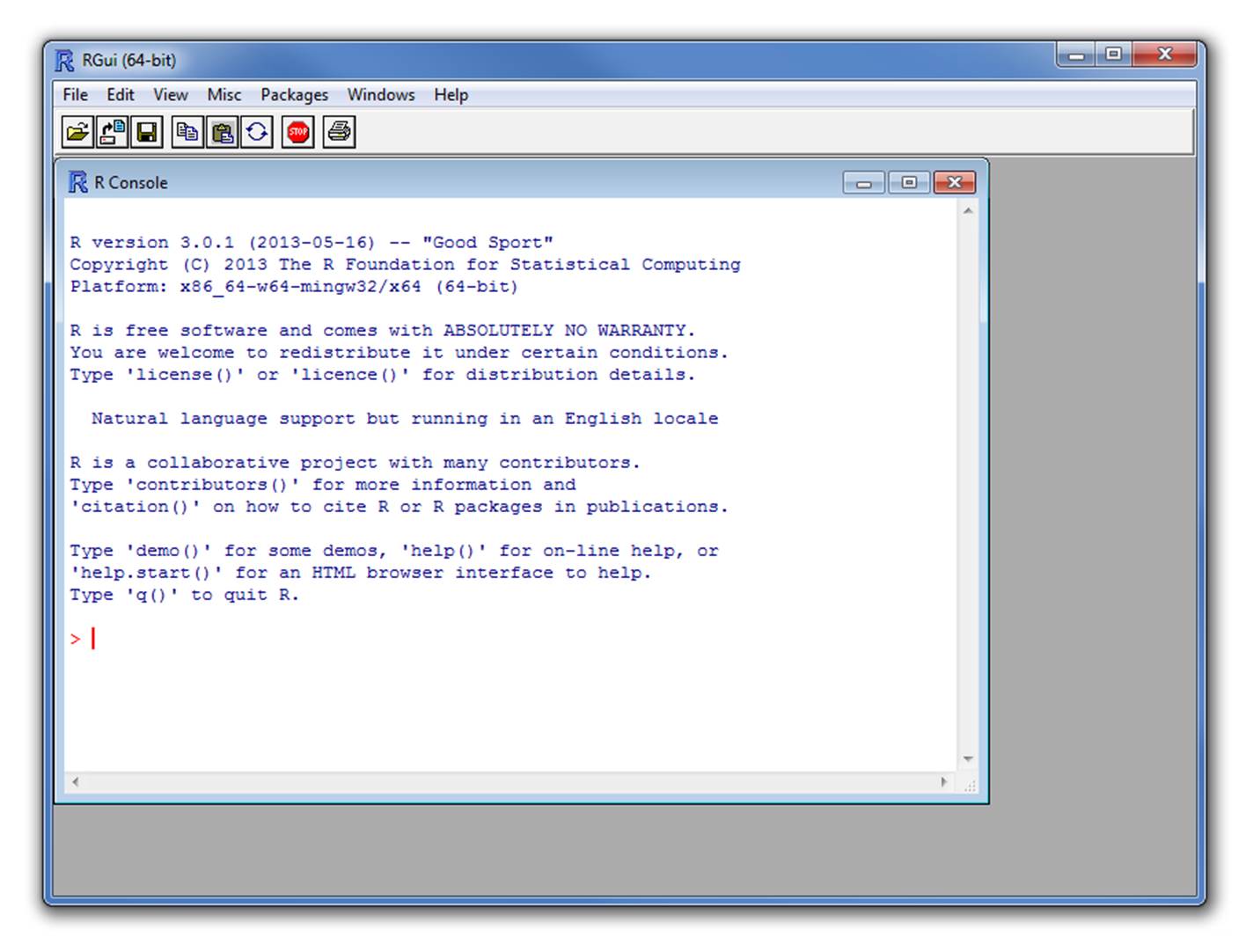
| 15:55, 3 December 2014 | 01-RConsole.jpg (file) |  | 123 KB | Aknop | (R-Console (R-GUI 3.0.1 64 bits version for windows)) | 1 |
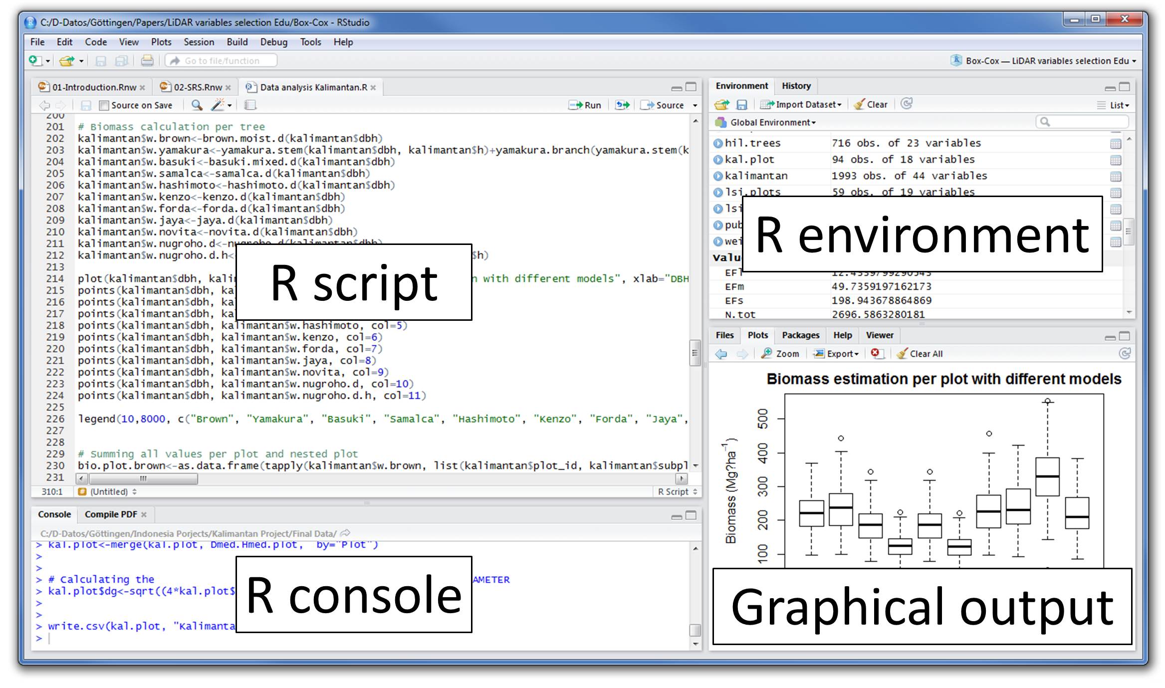
| 17:23, 3 December 2014 | 02-RStudio.jpg (file) |  | 377 KB | Aknop | (Interface of '''RStudio''' for Windows) | 1 |
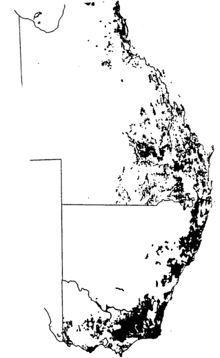
| 15:22, 18 January 2011 | 2.1.3.5-fig3.png (file) |  | 485 KB | Aspange | (Forest cover map of Eastern Australia (Bureau of Rural Resources 1991). At the boundary between the two provinces a marked change of the spatial arrangement of forest patches can be observed.) | 1 |
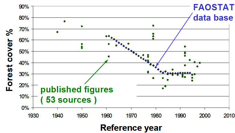
| 15:28, 18 January 2011 | 2.1.3.5-fig4.png (file) |  | 1.09 MB | Aspange | (Comparing published forest cover figures for Costa Rica from different sources (Kleinn and Morales 2002).) | 1 |
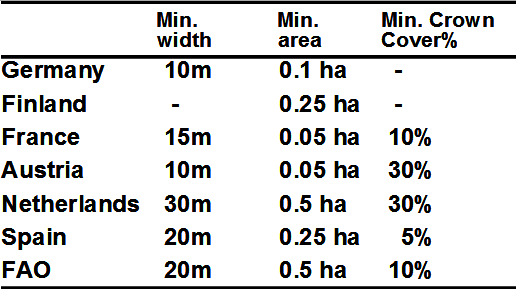
| 15:18, 18 January 2011 | 2.1.3.5-tab1.png (file) |  | 438 KB | Aspange | (Comparison of three quantitative criteria of forest definitions as used in some European countries NFI (EC 1996).) | 1 |
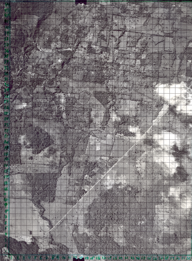
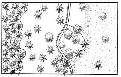
| 15:59, 18 January 2011 | 2.1.3.6-fig5.png (file) |  | 896 KB | Aspange | (Subdivision of a region into equal size cells for forest cover estimation. Reference: Kleinn C. 2000. Estimating metrics of forest spatial pattern from large area forest inventory cluster samples. Forest Science 46(4):548-557.) | 1 |
| 16:02, 18 January 2011 | 2.1.3.6-fig6.png (file) |  | 1.5 MB | Aspange | (Subdivision of a region into equal size cells for forest cover estimation. Reference: Kleinn C. 2000. Estimating metrics of forest spatial pattern from large area forest inventory cluster samples. Forest Science 46(4):548-557.) | 1 |
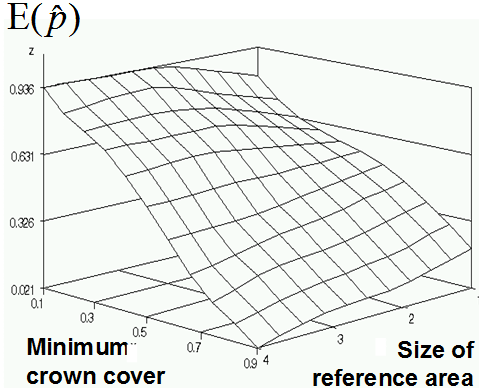
| 16:23, 18 January 2011 | 2.1.3.6-fig7.png (file) |  | 549 KB | Aspange | (Graphical illustration of the data presented in table 1. Reference: Kleinn C. 2000. Estimating metrics of forest spatial pattern from large area forest inventory cluster samples. Forest Science 46(4):548-557.) | 1 |
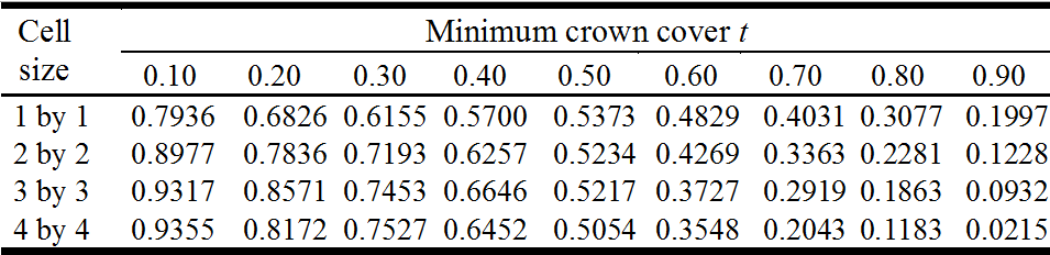
| 16:20, 18 January 2011 | 2.1.3.6-tab2.png (file) | 650 KB | Aspange | (Relationship between minimum crown cover percent, reference skill size and forest cover estimates. Reference: Kleinn C. 2000. Estimating metrics of forest spatial pattern from large area forest inventory cluster samples. Forest Science 46(4):548-557.) | 1 | |
| 17:40, 8 February 2011 | 2.1.4-fig8.png (file) |  | 105 KB | Aspange | (Some definitions of forest boundary Reference: Kenneweg, H. 2002. Neue methodische Ansätze zur Fernerkundung in den Bereichen Landschaft, Wald und räumliche Planung. In: Dech S et al. (Hrsg.): Tagungsband 19. GFD-Nutzerseminar, 15.-16. Okt. 2002, S. ) | 1 |
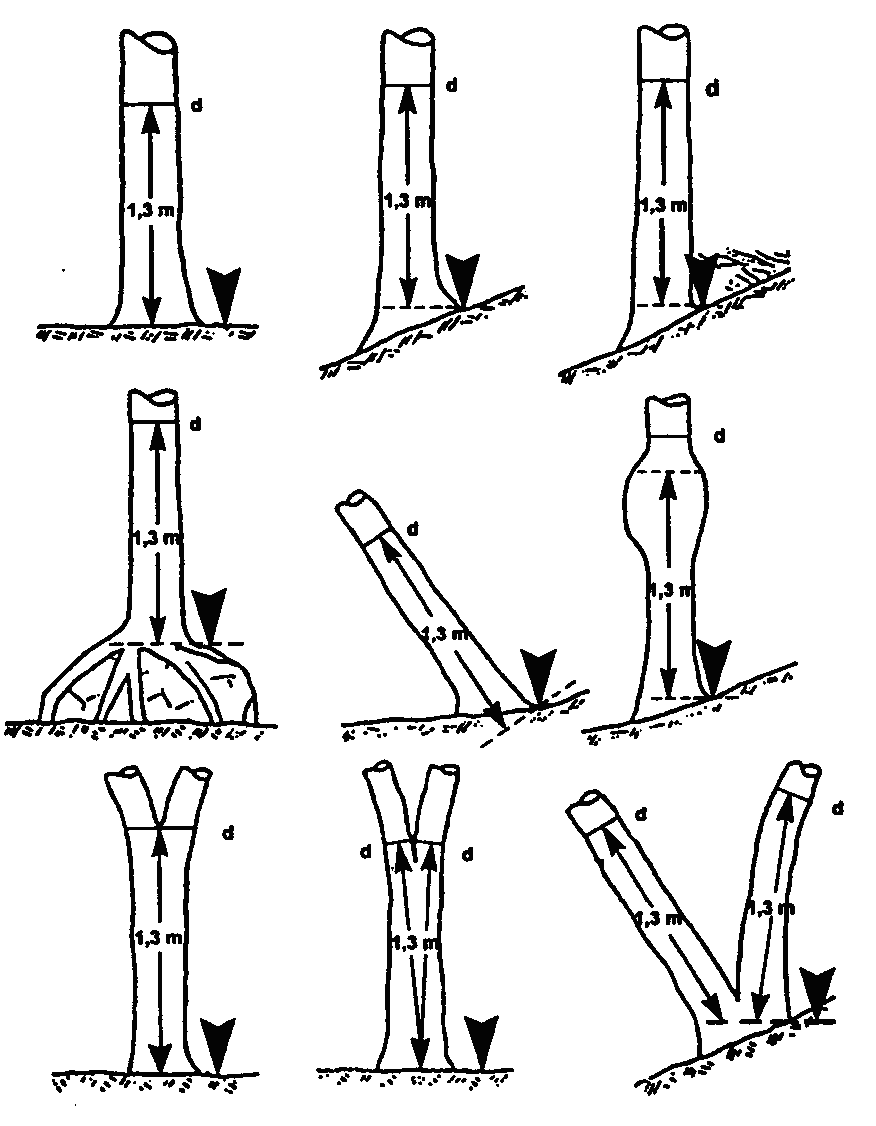
| 18:55, 8 February 2011 | 2.2.2-fig9.png (file) |  | 967 KB | Aspange | (Illustration of an instruction for dbh measurements. This example is taken from the field manual of the second national forest inventory in Germany. Reference: BMELV. 2007. Survey Instructions for the 2nd National Forest Inventory (2001-2002). Reprint F) | 1 |
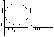
| 19:23, 8 February 2011 | 2.2.3.1-fig10.png (file) |  | 23 KB | Aspange | (Principle of ''dbh'' measurement with a caliper Reference: Kleinn, C. 2007. Lecture Notes for the Teaching Module Forest Inventory. Department of Forest Inventory and Remote Sensing. Faculty of Forest Science and Forest Ecology, Georg-August-Universit�) | 1 |
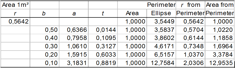
| 19:59, 8 February 2011 | 2.2.3.2-tab3.png (file) |  | 734 KB | Aspange | (Illustration of the effect of assuming a perfect circular cross section when determining basal area and dbh by tape-measurements. Reference: Kleinn, C. 2007. Lecture Notes for the Teaching Module Forest Inventory. Department of Forest Inventory and Remo) | 1 |
| 18:51, 17 February 2011 | 2.2.5.2-fig11.png (file) |  | 157 KB | Aspange | (The Finn caliper: fixed on a pole the tree diameter can be read up to a height of 7m. Reference: Keller M. (ed.). 2005. Schweizerisches Landesforstinventar. Anleitung für die Feldaufnahmen der Erhebung 2004-2007.) | 2 |
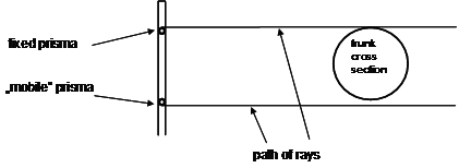
| 19:08, 17 February 2011 | 2.2.5.3-fig12.png (file) |  | 64 KB | Aspange | (Measurement rinciple of an optical caliper like Wheeler's pentaprism. Reference: Kleinn, C. 2007. Lecture Notes for the Teaching Module Forest Inventory. Department of Forest Inventory and Remote Sensing. Faculty of Forest Science and Forest Ecology, G) | 1 |
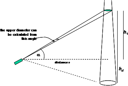
| 19:33, 17 February 2011 | 2.2.6-fig13.png (file) |  | 111 KB | Aspange | (Geometric principle of an optical caliper based on the measurement of an angle. Reference: Kleinn, C. 2007. Lecture Notes for the Teaching Module Forest Inventory. Department of Forest Inventory and Remote Sensing. Faculty of Forest Science and Forest ) | 1 |
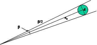
| 19:36, 17 February 2011 | 2.2.6-fig14.png (file) |  | 54 KB | Aspange | (In order to determine the diameter, the angle <math>\beta</math> and the distance <math>e_s</math> need to be determined. Reference: Kleinn, C. 2007. Lecture Notes for the Teaching Module Forest Inventory. Department of Forest Inventory and Remote Sensi) | 1 |
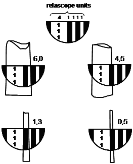
| 19:51, 17 February 2011 | 2.2.7-fig15.png (file) |  | 85 KB | Aspange | (Relascope units in the mirror relascope. The units are on a micro scale which adjusts automatically to slope; that is, the scale becomes more and more narrower with increasing deviation from the horizontal. By that construction principle it is guaranteed ) | 1 |
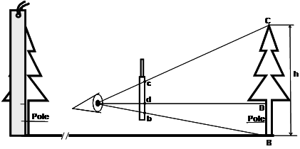
| 20:54, 17 February 2011 | 2.3.4-fig20.png (file) |  | 87 KB | Aspange | (Height meter of Christen which utilizes the geo-metric principle of height measurements. Reference: Kleinn, C. 2007. Lecture Notes for the Teaching Module Forest Inventory. Department of Forest Inventory and Remote Sensing. Faculty of Forest Science an) | 2 |
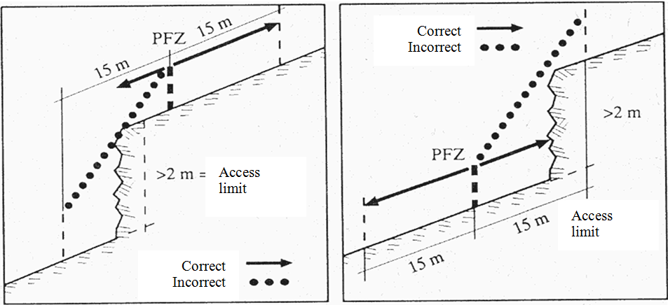
| 21:58, 17 February 2011 | 2.5-fig21.png (file) |  | 1.19 MB | Aspange | (Uneven oblique plane as used in Field Manual 2nd Swiss NFI. Reference: Brändli UB, A Herold, H Stierlin und J Zinggeler. 1994. Schweizerisches Landesforstinventar. Anleitung für die Feldaufnahmen der Erhebung 1993-1995. Birmensdorf, Eidg. Forschungsan) | 2 |
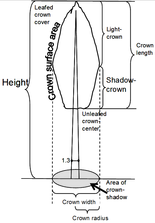
| 22:31, 17 February 2011 | 2.6.3-fig23.png (file) |  | 1.2 MB | Aspange | (Illustration of some crown attributes. Reference: Kramer, H. and Akca, A. 1995. Leitfaden zur Waldmesslehre. 3rd Edition. J.D. Sauerländers Verlag, Frankfurt. 266p.) | 1 |
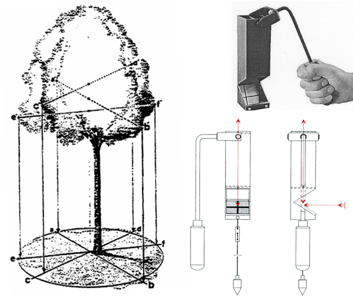
| 22:34, 17 February 2011 | 2.6.3-fig24.png (file) |  | 1.17 MB | Aspange | (''Left:'' Projection of a tree crown. ''Right:'' Crown mirror - Device to measure tree crown projection. Reference: Kleinn, C. 2007. Lecture Notes for the Teaching Module Forest Inventory. Department of Forest Inventory and Remote Sensing. Faculty of F) | 1 |
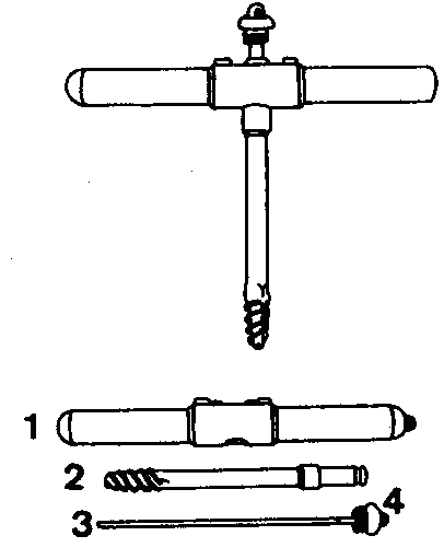
| 22:51, 17 February 2011 | 2.6.4-fig25.png (file) |  | 204 KB | Aspange | (Increment borer. Reference: Kleinn, C. 2007. Lecture Notes for the Teaching Module Forest Inventory. Department of Forest Inventory and Remote Sensing. Faculty of Forest Science and Forest Ecology, Georg-August-Universität Göttingen. 164 S.) | 1 |
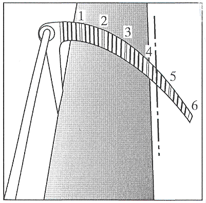
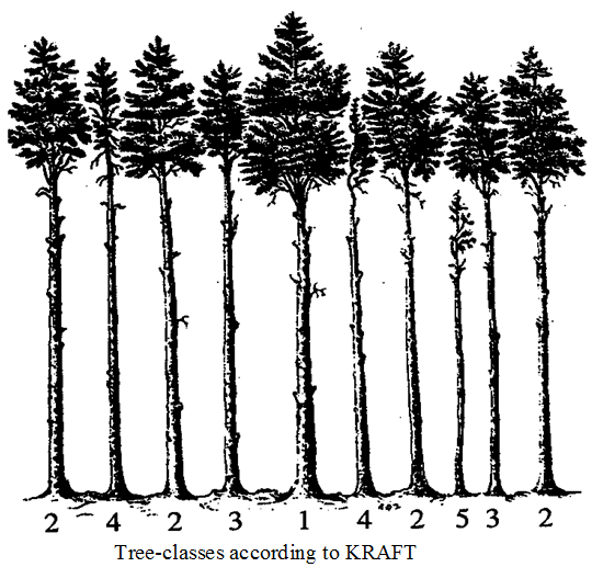
| 16:37, 18 February 2011 | 2.6.6-fig26.png (file) |  | 820 KB | Aspange | (''1'' predominant ''2'' dominant ''3'' co-dominant ''4'' dominated ''5'' falling behind (according to Kraft)) | 1 |
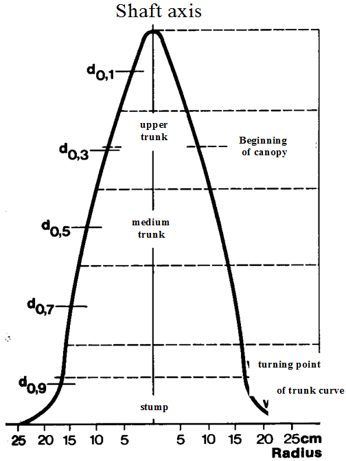
| 17:09, 18 February 2011 | 2.6.7.2-fig27.png (file) |  | 993 KB | Aspange | (Example of a taper curve characterizing the shape of a stem.) | 1 |
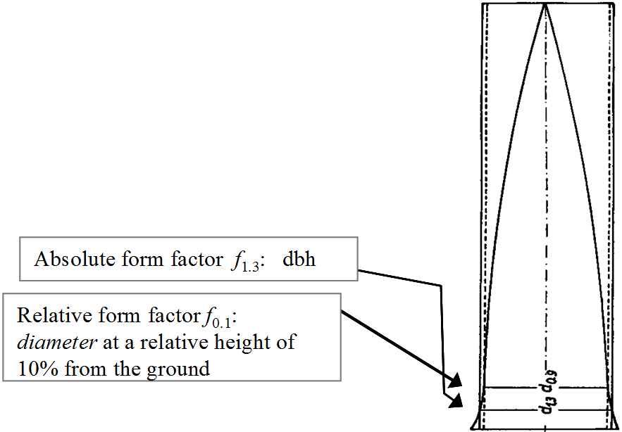
| 17:25, 18 February 2011 | 2.6.7.2-fig28.png (file) |  | 1.55 MB | Aspange | (Absolute ans relative form factor measurment.) | 1 |
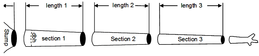
| 18:20, 18 February 2011 | 2.7.2.2-fig29.png (file) | 513 KB | Aspange | (Subdivision of a stem into sections.) | 1 | |
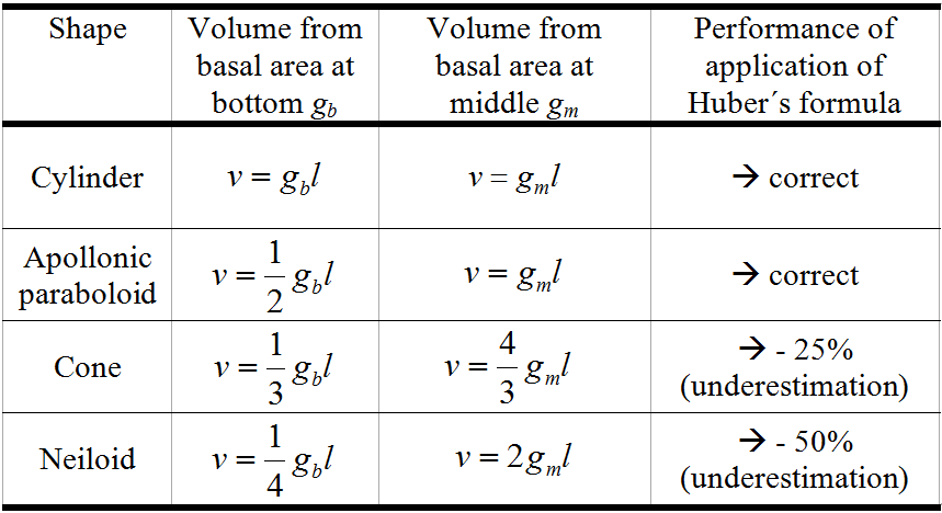
| 18:25, 18 February 2011 | 2.7.2.2-fig30.png (file) |  | 1.15 MB | Aspange | (The four basic geometric solids for sectionwise volume calculation. Reference: Kleinn, C. 2007. Lecture Notes for the Teaching Module Forest Inventory. Department of Forest Inventory and Remote Sensing. Faculty of Forest Science and Forest Ecology, Geor) | 1 |
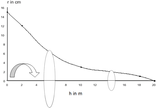
| 18:36, 18 February 2011 | 2.7.2.3-fig31.png (file) |  | 773 KB | Aspange | (Illustration of a taper curve which models the stem shape from the tree bottom (left) to the top (right). The radius is given as a function of tree height/stem length. By rotating this curve, we obtain a solid which is a model for the stem from which the ) | 1 |
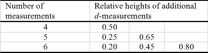
| 18:52, 18 February 2011 | 2.7.2.3-tab4.png (file) | 373 KB | Aspange | („Optimal“ distribution of measurement points along a stem to determine stem volume with highest precision by interpolation with cubic splines. Three measurement points are “fixed”: at 0.2 m height (assumed felling height), at 1.3 m (dbh) and total) | 1 | |
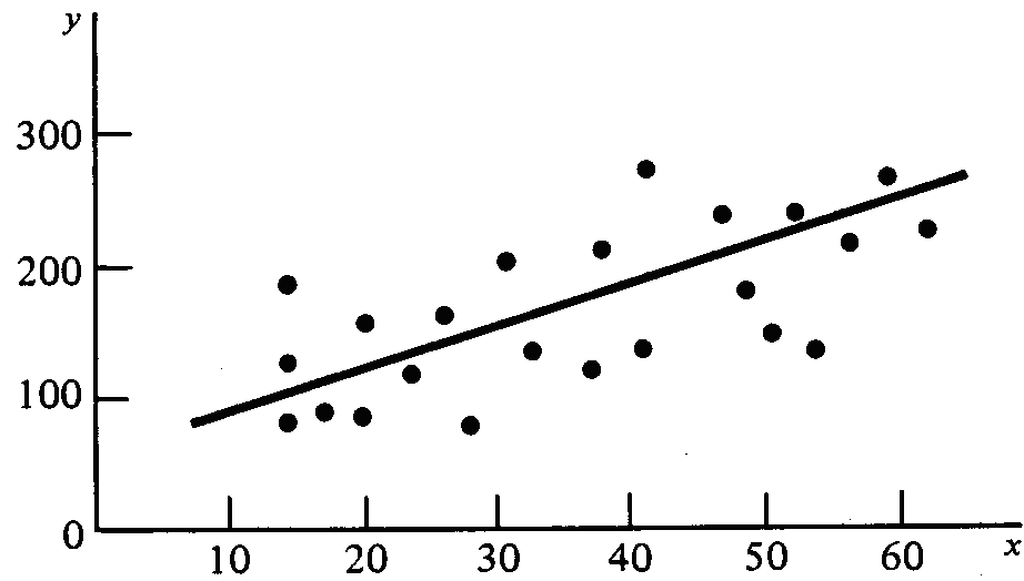
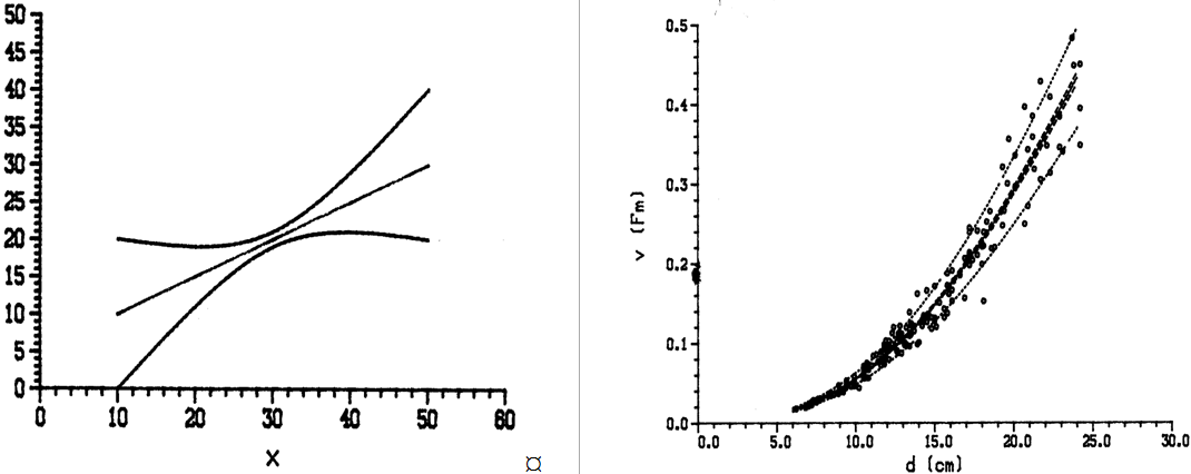
| 19:26, 18 February 2011 | 2.8.2-fig32.png (file) |  | 474 KB | Aspange | (Straight line representing a linear regression model between variable ''X'' and ''Y''.) | 1 |
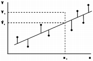
| 19:41, 18 February 2011 | 2.8.2-fig33.png (file) |  | 175 KB | Aspange | (Illustration of the least squares technique. The distance which is squared is not the perpendicular one but the distance in <math>y</math>-direction as we are interested in predictions over given values of <math>x</math>.) | 2 |
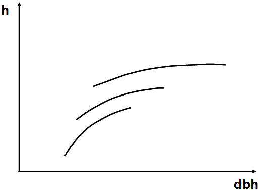
| 20:07, 18 February 2011 | 2.8.3-fig34.png (file) |  | 568 KB | Aspange | (Height curves in even aged stands exhibit typical changes over time which are depicted here simplified and schematically: they get flatter, shift right on the dbh axis and up on the height axis and cover a wider range of diameters (“become longer”).) | 1 |
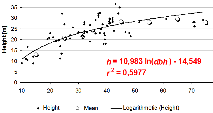
| 20:08, 18 February 2011 | 2.8.3-fig35.png (file) |  | 825 KB | Aspange | (Simple linear regression with ln(dbh) as sole independent variable. In addition to the data points, the mean heights per 10cm dbh-class are given. In this case, the model is obviously not flexible enough to adjust well to the height values for very large ) | 1 |
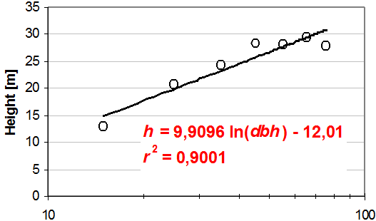
| 20:14, 18 February 2011 | 2.8.3-fig36.png (file) |  | 480 KB | Aspange | (The same height curve as in Figure 2 but drawn in a grid with ln(''dbh'') on the abscissa instead of ''dbh'' only.) | 1 |
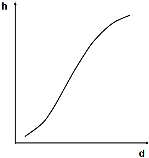
| 21:23, 18 February 2011 | 2.8.3-fig37.png (file) |  | 774 KB | Aspange | (A typical height curve in a natural uneven-aged stand. If the forest is in a “steady state”, This curve does not change over time and can simultaneously be interpreted as growth curve. Reference: Prodan M., R. Peters, F. Cox and P. Real. 1997.Mensur) | 1 |
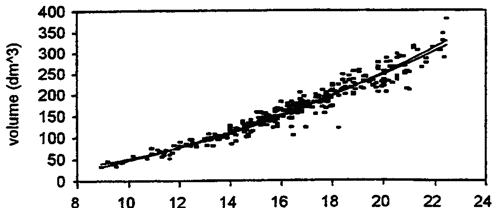
| 21:53, 18 February 2011 | 2.8.4-fig38.png (file) |  | 425 KB | Aspange | 1 | |
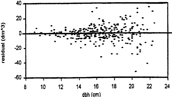
| 22:46, 1 March 2011 | 2.8.4-fig39.png (file) |  | 596 KB | Aspange | (Residual plot of residual volume (<math>dm^3</math> as Y-axis and ''dbh'' (cm) as X-axis showing unequal variance across ''dbh'' classes Reference: Kleinn, C. 2007. Lecture Notes for the Teaching Module Forest Inventory. Department of Forest Inventory ) | 1 |
| 22:58, 1 March 2011 | 2.8.4-fig40.png (file) |  | 1.31 MB | Aspange | (Schematic graphs of confidence intervals for the case of equal variances (left) and the unequal variances case as it presents itself with volume functions (right). Reference: Kleinn, C. 2007. Lecture Notes for the Teaching Module Forest Inventory. Depar) | 1 |
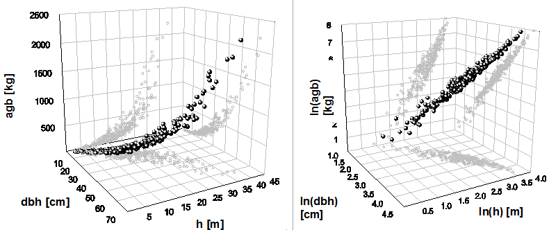
| 00:43, 2 March 2011 | 2.8.5-fig42.png (file) |  | 770 KB | Aspange | (Relationship between dbh, tree height and aboveground biomass on a metric (original) scale (left) and after logarithmic transformation of the variables (right) Reference: Kleinn, C. 2007. Lecture Notes for the Teaching Module Forest Inventory. Departmen) | 1 |
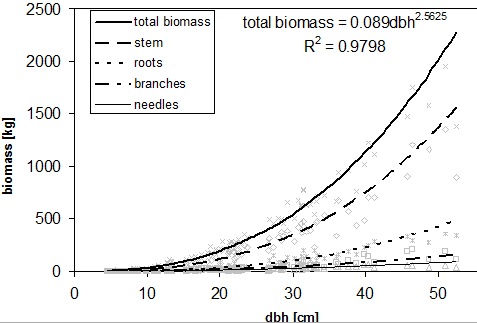
| 00:45, 2 March 2011 | 2.8.5-fig43.png (file) |  | 452 KB | Aspange | (Allometric functions for different tree compartments and total biomass for a Norway spruce dataset. Reference: Kleinn, C. 2007. Lecture Notes for the Teaching Module Forest Inventory. Department of Forest Inventory and Remote Sensing. Faculty of Forest ) | 1 |
| 13:12, 8 November 2012 | 2012-11 Göttingen Freiberg.pdf (file) | 383 KB | Fehrmann | 1 | ||
| 12:39, 4 December 2012 | 2012-11 Göttingen Kanninen.pdf (file) | 2.48 MB | Schreiner | 1 | ||
| 16:20, 7 November 2012 | 2012-11 Göttingen REDD driver.pdf (file) | 1.58 MB | Fehrmann | (Presentation given by Timm Tennigkeit, UNIQUE forestry and land use GmbH in context of the introduction seminar to the DAAD FD6 Workshop) | 1 | |
| 11:52, 5 December 2012 | 2012-11 Göttingen Stoll.pdf (file) | 1.12 MB | Schreiner | 1 | ||
| 11:54, 5 December 2012 | 2012-11 Göttingen Tennigkeit.pdf (file) | 1.96 MB | Schreiner | 1 | ||
| 16:49, 29 January 2014 | 2014-01 Göttingen Kanninen.pdf (file) | 1.71 MB | Fehrmann | (Presentation given by Prof. Dr. M. Kanninen.) | 1 | |
| 13:32, 30 June 2015 | 2015-06-11 German NFI Instrument for Data Provison Kaendler.pdf (file) | 2.42 MB | Schreiner | 1 | ||
| 13:33, 30 June 2015 | 2015-06-11 Operationalizing REDD Carodenuto.pdf (file) | 2.9 MB | Schreiner | 1 | ||
| 17:45, 8 September 2015 | 2015-06-11 PROMOTING NATIONAL FOREST INVENTORIES - FAO'S LESSONS LEARNED Morales.pdf (file) | 2.96 MB | Schreiner | 2 |
First page |
Previous page |
Next page |
Last page |