File list
This special page shows all uploaded files. When filtered by user, only files where that user uploaded the most recent version of the file are shown.
| Name | Thumbnail | Size | User | Description | Versions | |
|---|---|---|---|---|---|---|
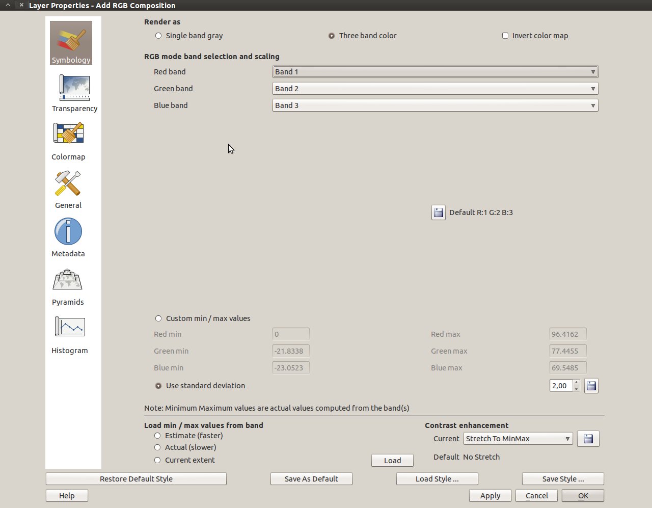
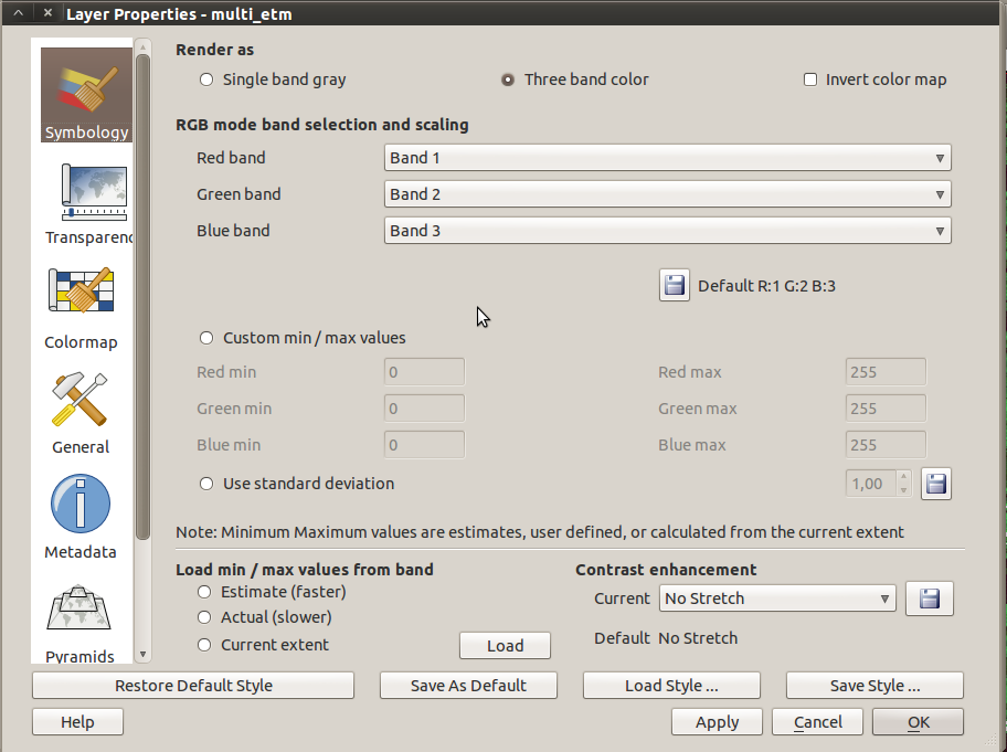
| 17:40, 17 February 2011 | QGIS RGB dialog.jpg (file) |  | 93 KB | Lburgr | (Screenshot of the QGIS raster layer properties RGB option (in Ubuntu). ) | 1 |
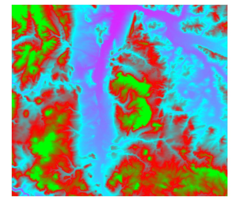
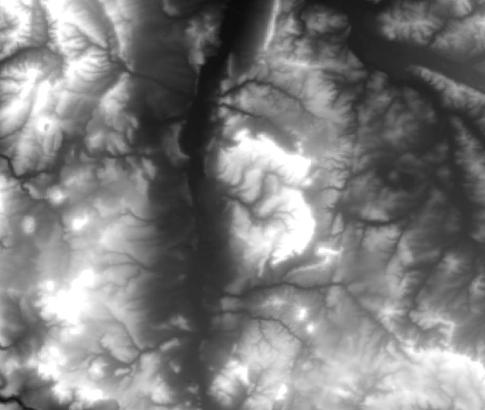
| 14:33, 17 February 2011 | Dem freak.jpg (file) |  | 93 KB | Lburgr | (A digital elevation model displayed with the QGIS “freak out” option.) | 1 |
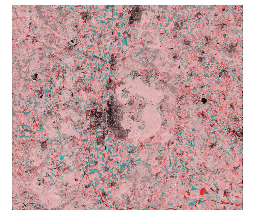
| 16:18, 13 February 2011 | Ndvi 92 to 05.jpg (file) |  | 196 KB | Lburgr | (A multitemporal color composite created in GRASS with r.composite.) | 1 |
| 16:17, 13 February 2011 | Change NDVI 92 05 comp.jpg (file) |  | 266 KB | Lburgr | (A multitemporal color composite created in GRASS and exported to tif-format. Inadequate symbology.) | 1 |
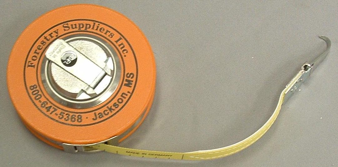
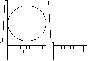
| 20:14, 8 February 2011 | Diameter tape.png (file) |  | 1.66 MB | Aspange | (Example für a diameter tape. Reference: treecaresupplies.com) | 1 |
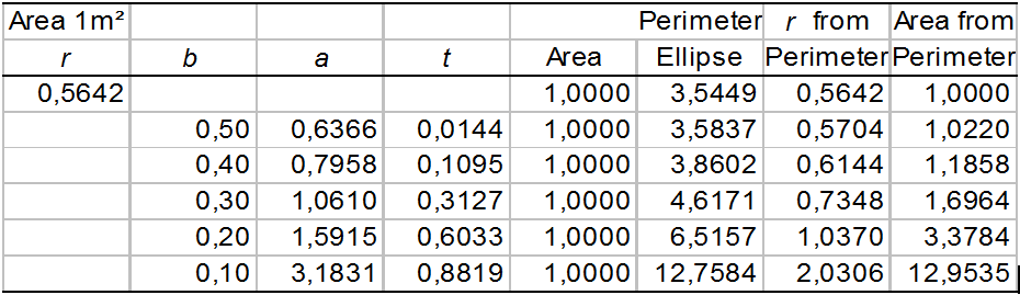
| 19:59, 8 February 2011 | 2.2.3.2-tab3.png (file) |  | 734 KB | Aspange | (Illustration of the effect of assuming a perfect circular cross section when determining basal area and dbh by tape-measurements. Reference: Kleinn, C. 2007. Lecture Notes for the Teaching Module Forest Inventory. Department of Forest Inventory and Remo) | 1 |
| 19:23, 8 February 2011 | 2.2.3.1-fig10.png (file) |  | 23 KB | Aspange | (Principle of ''dbh'' measurement with a caliper Reference: Kleinn, C. 2007. Lecture Notes for the Teaching Module Forest Inventory. Department of Forest Inventory and Remote Sensing. Faculty of Forest Science and Forest Ecology, Georg-August-Universit�) | 1 |
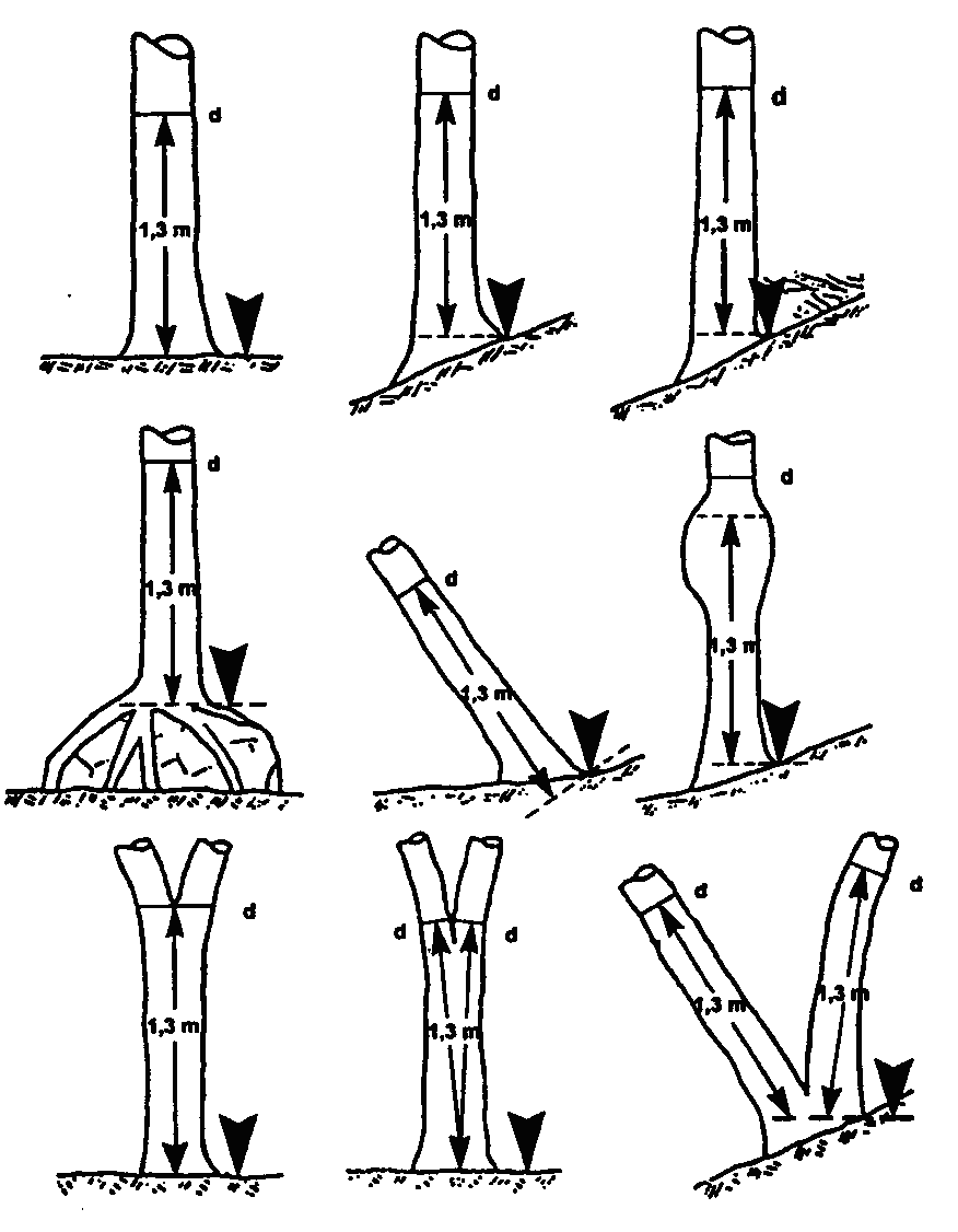
| 18:55, 8 February 2011 | 2.2.2-fig9.png (file) |  | 967 KB | Aspange | (Illustration of an instruction for dbh measurements. This example is taken from the field manual of the second national forest inventory in Germany. Reference: BMELV. 2007. Survey Instructions for the 2nd National Forest Inventory (2001-2002). Reprint F) | 1 |
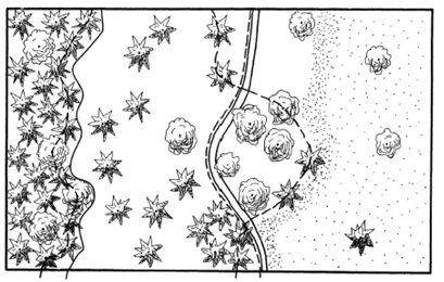
| 17:40, 8 February 2011 | 2.1.4-fig8.png (file) |  | 105 KB | Aspange | (Some definitions of forest boundary Reference: Kenneweg, H. 2002. Neue methodische Ansätze zur Fernerkundung in den Bereichen Landschaft, Wald und räumliche Planung. In: Dech S et al. (Hrsg.): Tagungsband 19. GFD-Nutzerseminar, 15.-16. Okt. 2002, S. ) | 1 |
| 16:21, 26 January 2011 | Dem pseudo.jpg (file) |  | 97 KB | Lburgr | (A digital elevation model displayed in pseudocolor.) | 1 |
| 16:20, 26 January 2011 | Dem grey.jpg (file) |  | 60 KB | Lburgr | (A digital elevation model displayed in greyscale.) | 1 |
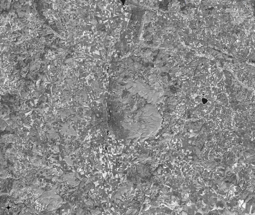
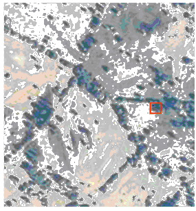
| 13:52, 26 January 2011 | Etm40 grey stdev.jpg (file) |  | 267 KB | Lburgr | (Fourth band of a LANDSAT image symbolized in greyscale; based on a standard deviaton of 2.5 with stretch to MinMax in QGIS.) | 1 |
| 13:51, 26 January 2011 | Etm40 grey.jpg (file) |  | 214 KB | Lburgr | (Fourth band of a LANDSAT image symbolized in grey scale.) | 1 |
| 18:45, 25 January 2011 | Raster properties.png (file) |  | 109 KB | Lburgr | (A screenshot of the QGIS 1.6 rastermap properties dialog.) | 1 |
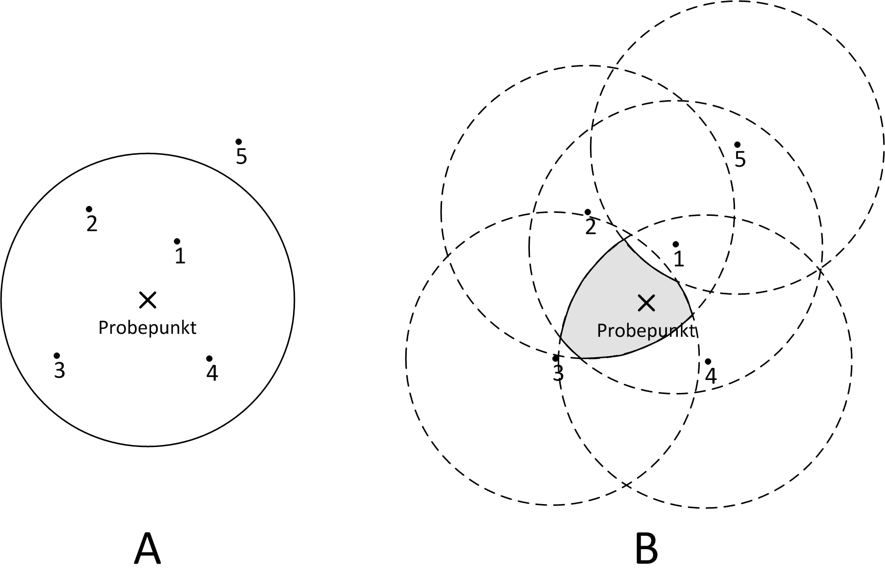
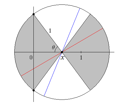
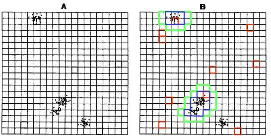
| 16:38, 20 January 2011 | InclusionZones.png (file) |  | 59 KB | Fehrmann | 1 | |
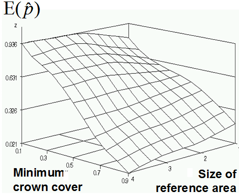
| 16:23, 18 January 2011 | 2.1.3.6-fig7.png (file) |  | 549 KB | Aspange | (Graphical illustration of the data presented in table 1. Reference: Kleinn C. 2000. Estimating metrics of forest spatial pattern from large area forest inventory cluster samples. Forest Science 46(4):548-557.) | 1 |
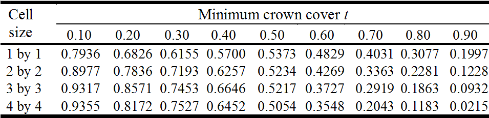
| 16:20, 18 January 2011 | 2.1.3.6-tab2.png (file) | 650 KB | Aspange | (Relationship between minimum crown cover percent, reference skill size and forest cover estimates. Reference: Kleinn C. 2000. Estimating metrics of forest spatial pattern from large area forest inventory cluster samples. Forest Science 46(4):548-557.) | 1 | |
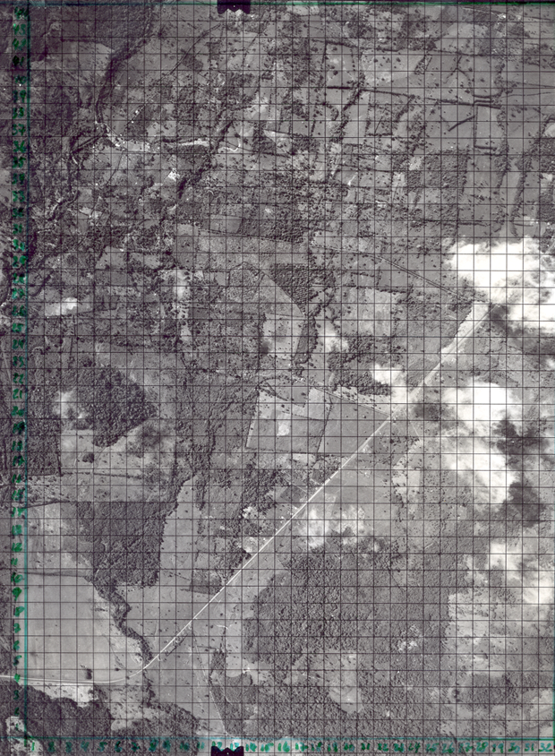
| 16:02, 18 January 2011 | 2.1.3.6-fig6.png (file) |  | 1.5 MB | Aspange | (Subdivision of a region into equal size cells for forest cover estimation. Reference: Kleinn C. 2000. Estimating metrics of forest spatial pattern from large area forest inventory cluster samples. Forest Science 46(4):548-557.) | 1 |
| 15:59, 18 January 2011 | 2.1.3.6-fig5.png (file) |  | 896 KB | Aspange | (Subdivision of a region into equal size cells for forest cover estimation. Reference: Kleinn C. 2000. Estimating metrics of forest spatial pattern from large area forest inventory cluster samples. Forest Science 46(4):548-557.) | 1 |
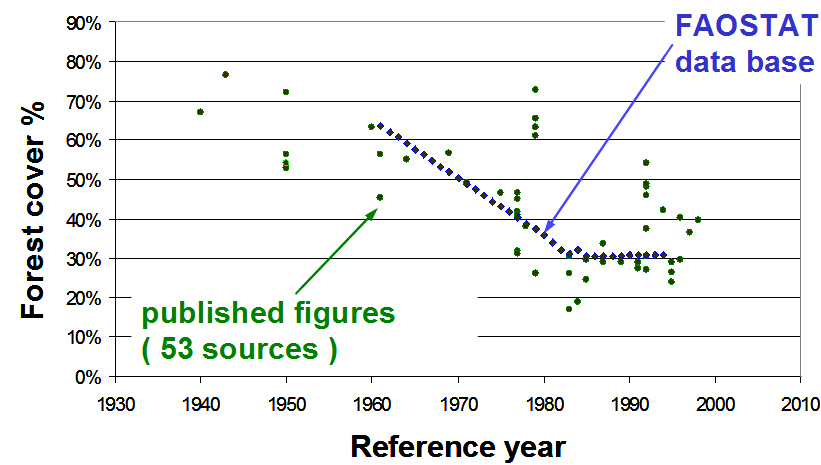
| 15:28, 18 January 2011 | 2.1.3.5-fig4.png (file) |  | 1.09 MB | Aspange | (Comparing published forest cover figures for Costa Rica from different sources (Kleinn and Morales 2002).) | 1 |
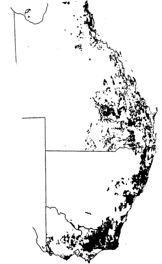
| 15:22, 18 January 2011 | 2.1.3.5-fig3.png (file) |  | 485 KB | Aspange | (Forest cover map of Eastern Australia (Bureau of Rural Resources 1991). At the boundary between the two provinces a marked change of the spatial arrangement of forest patches can be observed.) | 1 |
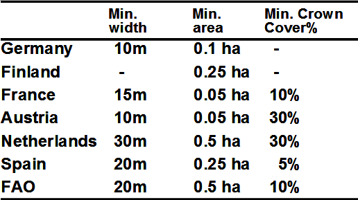
| 15:18, 18 January 2011 | 2.1.3.5-tab1.png (file) |  | 438 KB | Aspange | (Comparison of three quantitative criteria of forest definitions as used in some European countries NFI (EC 1996).) | 1 |
| 14:44, 18 January 2011 | Buffon's needle corrected.PNG (file) |  | 9 KB | Fehrmann | (Taken from Wikipedia.) | 1 |
| 16:19, 17 January 2011 | Exercise.png (file) |  | 6 KB | Fehrmann | (Symbol for exercises) | 1 |
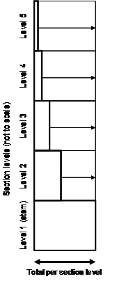
| 19:07, 7 January 2011 | SkriptFig 103.jpg (file) |  | 40 KB | Fheimsch | (Illustration of estimation in randomized branch sampling (after Good et al. 2001): for each section level, the observed value (bold rectangle) is expanded to an estimated total value by dividing that value by its selection probability which is indicated h) | 1 |
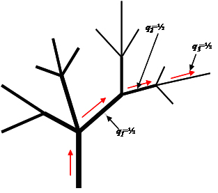
| 18:55, 7 January 2011 | SkriptFig 102.jpg (file) |  | 45 KB | Fheimsch | (Illustration of randomized branch sampling. The path selected here follows the arrows along the branches. For each section its specific selection probability is determined by the random selection carried out at its starting point. The overall selection pr) | 1 |
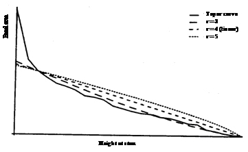
| 21:29, 6 January 2011 | SkriptFig 101.jpg (file) |  | 41 KB | Fheimsch | (Plot of height at stem against basal area.) | 1 |
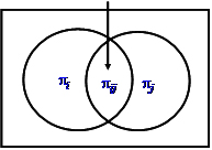
| 15:28, 6 January 2011 | SkriptFig 100.jpg (file) |  | 34 KB | Fheimsch | (Diagram illustrating the joint inclusion probability.) | 1 |
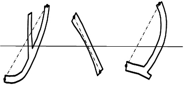
| 18:07, 4 January 2011 | SkriptFig 98.jpg (file) |  | 40 KB | Fheimsch | (If line intersect sampling is used as a tool to select sample objects, a “needle” is to be defined on each object. Only intersection of the sample line with this needle leads to the selection of that object.) | 1 |
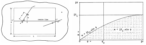
| 17:07, 4 January 2011 | SkriptFig 97.jpg (file) |  | 60 KB | Fheimsch | (Intersection probability as a function of the orientation of the needle and the distance of the needle to the nearest line (from deVries 1986)) | 1 |
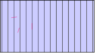
| 16:34, 4 January 2011 | SkriptFig 96.jpg (file) |  | 47 KB | Fheimsch | (Illustration of Buffon´s needle problem: the probability is to be estimated that a needle intersects with one of the parallel lines.) | 1 |
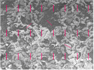
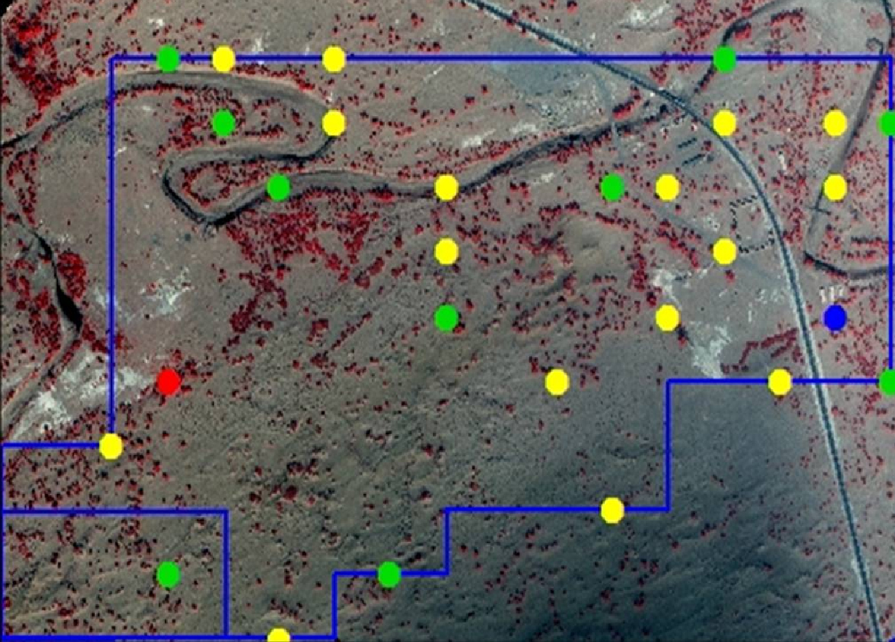
| 15:54, 4 January 2011 | SkriptFig 95.jpg (file) |  | 125 KB | Fheimsch | (Application of line intercept sampling on an aerial photograph.) | 1 |
| 15:02, 4 January 2011 | SkiptFig 94.jpg (file) |  | 875 KB | Fheimsch | (Section of a “riparian forest” along river Tarim in North-Western China. Here, a stratification along crown cover can hard-ly be done by delineation and pre-stratification but double sampling for stratification appeared more suitable. The differently ) | 1 |
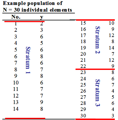
| 00:42, 30 December 2010 | 5.2.6-fig75.png (file) |  | 490 KB | Aspange | (Sub-dividing the example population (arbitrarily) in three strata, for illustration purposes. Reference: Kleinn, C. 2007. Lecture Notes for the Teaching Module Forest Inventory. Department of Forest Inventory and Remote Sensing. Faculty of Forest Scienc) | 8 |
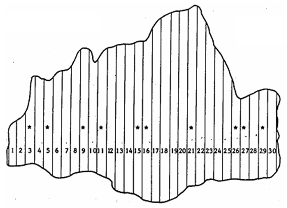
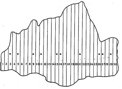
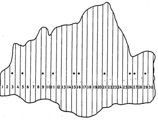
| 20:37, 29 December 2010 | 5.6.1-fig93.png (file) |  | 687 KB | Aspange | (Example of a population of 30 unequally sized strip plots; here, the ratio estimator may be applied for estimation using plot size as co-variable (DeVries 1986). Reference: de Vries 1986<ref>de Vries, P.G., 1986. Sampling Theory for Forest Inventory. A ) | 1 |
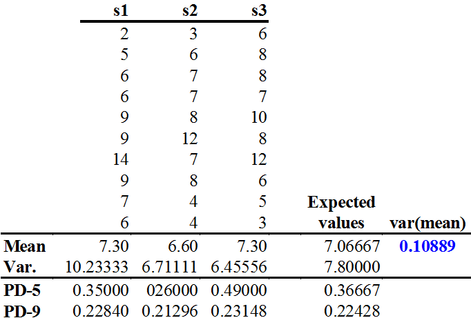
| 14:36, 23 December 2010 | 5.5.6.4-tab19.png (file) |  | 923 KB | Aspange | (The population of all possible systematic samples of size <math>n=10</math> drawn from the example population. There are only 3 possibilities. PD-5 and 9 are the estimated error variances from the pair differences method with 5 non-overlapping and 9 overl) | 2 |
| 14:14, 23 December 2010 | 5.6-fig93.png (file) |  | 118 KB | Aspange | (Example population of 30 unequally sized strip plots; here, the ratio estimator may be apllied for estimation using plot size as covariable (de Vries 1986) Reference: de Vries, P.G., 1986. Sampling Theory for Forest Inventory. A Teach-Yourself Course. S) | 1 |
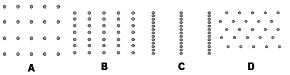
| 14:08, 23 December 2010 | 5.5.8-fig92.png (file) | 86 KB | Aspange | (Different patterns of systematic sample grids. A being a square grid, B being a rectangular grid with <math>a:b=2:1</math>, C being a rectangular grid with <math>a:b=8:1</math>, and D being a triangular grid as defined in Matérn (1960). Reference: Mat�) | 1 | |
| 13:12, 23 December 2010 | 5.5.6.4-fig91.png (file) |  | 139 KB | Aspange | (Building pairs of neighboring observations for the approximation of error variance in systematic sampling. Pairs can either be built “exclusively” (below) or overlapping (above). Reference: Kleinn, C. 2007. Lecture Notes for the Teaching Module For) | 1 |
| 13:07, 22 December 2010 | 5.5.5-fig90.png (file) |  | 314 KB | Aspange | (Two examples of the difference between random and fixed orientation grids. Left: squares of different side lengths (abscissa) are sampled with grid of unit size. Right: a forest map is sampled with random and fixed orientation grids of different width whe) | 1 |
| 12:50, 22 December 2010 | 5.5.3-fig89.png (file) |  | 68 KB | Aspange | (When a population is sub-divided into strata, systematic sampling always produces proportional allocation of plots. Reference: Kleinn, C. 2007. Lecture Notes for the Teaching Module Forest Inventory. Department of Forest Inventory and Remote Sensing. Fa) | 1 |
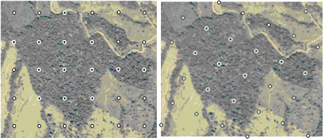
| 12:33, 22 December 2010 | 5.5.2-fig88.png (file) |  | 278 KB | Aspange | (One and the same grid randomly laid over the same area results in different numbers of sample points inside the forest area. Reference: Kleinn, C. 2007. Lecture Notes for the Teaching Module Forest Inventory. Department of Forest Inventory and Remote Se) | 1 |
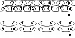
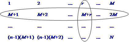
| 12:08, 22 December 2010 | 5.5.1-fig87.png (file) |  | 58 KB | Aspange | (Illustration of systematic sampling in terms of stratified sampling or cluster sampling. The population of <math>N</math> elements is arranged here in groups of <math>M</math>. Reference: Kleinn, C. 2007. Lecture Notes for the Teaching Module Forest Inv) | 1 |
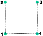
| 21:15, 16 December 2010 | 5.3.4-fig81.png (file) |  | 19 KB | Aspange | (Cluster plot design as used in a regional forest inventory in the NOrthern Zone of Costa Rica (Kleinn 1993). This design is used to illustrate approaches to area estimation.) | 1 |
| 19:59, 16 December 2010 | 5.1.3-fig73.png (file) |  | 78 KB | Aspange | 1 | |
| 19:17, 16 December 2010 | 5.2.6-fig74.png (file) |  | 98 KB | Aspange | 1 | |
| 23:34, 10 December 2010 | 5.4-fig86.png (file) |  | 87 KB | Aspange | 1 | |
| 21:13, 10 December 2010 | 5.4-fig85.png (file) |  | 446 KB | Aspange | 1 | |
| 17:48, 3 December 2010 | SkriptFig 73.jpg (file) |  | 64 KB | Fheimsch | (Figure 73. Example population) | 1 |
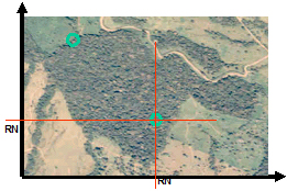
| 15:46, 3 December 2010 | SkriptFig 72.jpg (file) |  | 82 KB | Fheimsch | (Allocating a sample plot randomly in the displayed forest patch.) | 1 |
First page |
Previous page |
Next page |
Last page |