Ratio estimator

Revision as of 21:08, 29 December 2010

Languages:

English

Introduction

Figure 1 Example of a population of 30 unequally sized strip plots; here, the ratio estimator may be applied for estimation using plot size as co-variable (DeVries 1986^[1]).

There are situations in forest inventory sampling in which the value of the target variable is known (or suspected) to be highly correlated to an other variable (called co-variable or ancillary variable). We know from the discussion on spatial autocorrelation and the optimization of cluster plot design that correlation between two variables means essentially that the one variable does yet contain a certain amount of information about the other variable. The higher the correlation the better can the value of the second variable be predicted when the value of the first is known (and vice versa). Therefore, if such a co-variable is there on the plot, it would make sense to also observe it and utilize the correlation to the target variable to eventually improve the precision of estimating the target variable. This is exactly the situation where the ratio estimator is applied.

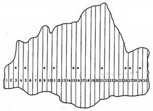
A typical and basic example is that of sample plots of unequal size, as depicted, for example in Figure 1 where strips of different length constitute the population of samples. Another example would be clusters of unequal size: while cluster sampling only deals with the case of clusters of equal size, the ratio estimator allows to take into account the differently sized sample plots. Here, obviously, the size of the sample plots is the co-variable that needs to be determined for each sample plot. That a high positive correlation is to be expected between most forestry-relevant attributes and plot size should be obvious: the larger the plot the more basal area, number of stems, volume etc. is expected to be present.

In fact, the ratio estimator does not introduce a new sampling technique: we use here the example of simple random sampling (as sampling design). The ratio estimator introduces new elements

1. into the plot design (observation of an ancillary variable on each plot, in addition to the observation of the target variable); and above all
2. into the estimation design; the ratio estimator integrates the ancillary variable into the estimator.

Side-comment:

For those who have some knowledge or interest (or both) on the design of experiments and the linear statistical models used there (analysis of variance) it might be interesting to note that also in the field of experimental design there is a technique in which a co-variable is observed on each experimental plot in order to allow a more precise estimation of the effects of treatments: this technique is called analysis of co-variance.

The ratio estimator is called ratio estimator because, what we actually estimate from the sample plot is a ratio: for example, number of stems per hectare. The ancillary variable (“area” in this case) appears always in the denominator of the ratio. We denote the variable of interest as usual with yi and the ancillary variable as xi; some more on notation is given in the following chapter.

Notation

\(R\,\)	Parametric ratio, that is the true ratio present in the population;
\(\mu_y\,\)	Parametric mean of the target variable \(Y\);
\(\mu_x\,\)	Parametric mean of the ancillary variable \(X\);
\(\tau_x\,\)	Parametric total of ancillary variable \(X\);
\(\rho\,\)	Parametric Pearson coefficient of correlation between \(Y\) and \(X\);
\(\sigma_y\,\)	Parametric standard deviation of the target variable \(Y\);
\(\sigma_x\,\)	Parametric standard deviation of ancillary variable \(X\);
\(n\,\)	Sample size;
\(r\,\)	Estimated ratio;
\(y_i\,\)	Value of the target variable observed on the \(i^{th}\) sampled element (plot);
\(x_i\,\)	Ancillary variable, e.g. area, for \(i^{th}\) plot;
\(\bar y\,\)	Estimated mean of target variable;
\(\bar x\,\)	Estimated mean of ancillary variable;
\(\hat{\tau}_y\,\)	Estimated total of target variable;
\(\hat{\rho}\,\)	Estimated coefficient of correlation of \(Y\) and \(X\);
\({s_y}^2\,\)	Estimated variance of target variable;
\({s_x}^2\,\)	Estimated variance of ancillary variable.

With the notation for the ratio estimator it should, above all, be observed, that the letters \(r\) and \(R\) are used here for ratio – and not for the correlation coefficient. That causes some times confusions. We use the Greek letter \(\rho\) (rho) for the parametric correlation coefficient and the usual notation for the estimation using the “hat” sign\[\hat{\rho}\].

References

sorry:

This section is still under construction! This article was last modified on 12/29/2010. If you have comments please use the Discussion page or contribute to the article!