Object-based classification (Tutorial)

sorry:

This section is still under construction! This article was last modified on 09/16/2014. If you have comments please use the Discussion page or contribute to the article!

This exercise is part of the QGIS Tutorial 2013/14

Determining segmentation parameters

1. Start Monteverdi
2. Open dataset in Monteverdi: File --> Open dataset e.g. 188_pca_indices_pan.tif
3. Subset data to a small area: File --> Extract ROI from dataset, in the field Image to read --> Reader0 select a file e.g. 188_pca_indices_pan.tif and press OK
4. Drag the mouse in the Select the ROI window to select a region equivalent to 500x500 pixels and press OK to make an output image. You can name it ExtractROI1. Not sure if this is to be the file name or a button pressed. - Levent (talk)
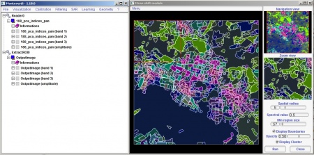
5. To perform the mean shift segmentation: Filtering --> Mean shift clustering, in the field Image to apply shift on select the output image from step 4. The Mean shift module window opens. Set the following parameters.
   • Spatial radius = 5
   • Spectral values = 0.5,
   • Min region size = 57.
   • Check the boxes Display Boundaries and Display cluster I assume these are check boxes? - Levent (talk)
6. Confirm with Run. An output named Labeled image is created (Figure A) Is this right? - Levent (talk).
7. Finally click Close to create all the output in Monteverdi window.

Figure A: Mean shift module in Monteverdi

Object labeling and segmentation via SVM

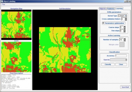
1. Object labeling: Go to Learning --> Object Labeling, in the field The image to classify select file generated in the previous step and in the field The segmentation of the image select file MeanShift1 --> Labeled Image and press OK Correct? - Levent (talk). A window Object Labeling opens.
2. Click Add to start object labeling. A new class appears in the Objects tab in the upper right corner of the window. Specify color red for New Class 0 = Urban. Double right click the image to select 10 urban objects as visually intepreted. Repeat the same procedure for New Class 1 = Cropland in yellow color and New Class 2 = Forest in green color.
3. To select shape and pixel parameters for object clustering: In the Features tab check STATS::Band1::Mean, STATS::Band2::Mean, STATS::Band3::Mean -- are these really the names of the boxes? - Levent (talk)
4. To selecti Support Vector Machine (SVM) parameters: Leave the other parameters to default and check the Parameters optimization box. Click classify to obtain the output displayed in Figure B. Using the Opacity slide, you can compare the output with the original image. Note the accuracy measure in the lower right side of the window.
5. Try other Features by checking them in the Features tab and compare output clusters with the output of parameters specified at step 3.

Info

For more detailed information on the SVM algorithm visit the library website

Figure B: Object labeling menu in Monteverdi

Object based segmentation by mean shift clustering

1. Load the raster map 188_pca_indices_pan.tif provided in the course data. Open Mean Shift Segmentation (Large scale, vector output) from the Orfeo toolbox algorithms in the Processing bar.
2. Select 188_pca_indices_pan.tif as input image. Change Range radius to 0.5 and Min Region size to 50. Specify the output file as Segments_all.shp and click RUN.
3. Load Segments_all.shp to the project. To view both the vector segments and the underlying image file, visualize the segments as hollow polygons: Right click on Segments_all.shp in the TOC, and select Properties --> Style and select Fill-Simple fill with No brush as Fill style. Change the border outline colour to white for better visibility (see figure C).
4. Split the multiband image 188_pca_indices_ pan_mean.tif to single band rasters. This step is necessary to allow extraction of individual segment spectral values using the zonal statistics tool as shown in step 5: Open Split image tool from the Orfeo toolbox. Select Image manipulation --> Split image and specify output image.
5. To extract pixel spectral data for each object using the Zonal statistics Plugin: Install Zonal Statistics Plugin from the Plugins --> Manage and Install plugins menu. Select Get more and browse for the Zonal statistics plugin. After successfully installing the tool, open it from Raster --> Zonal statistics --> Zonal statistics and specify the Raster layer, Polygon layer containing the zones and Output column for Bands 1, 2 and 3 respectively.
6. Rasterize the segments to prepare for classification: Open the Rasterization tool from the Orfeo tool box, selecting Vector Data Manipulation --> Rasterization. Select Segments_all.shp as Input vector dataset. Select 188_pca_indices_pan_mean.tif as Input reference image. Also enter the input coordinates Output Upper-left x and Output Upper-left y. The coordinates can be found in the Metadata tab of the layer Properties. Change Spacing (GSD)x and Spacing (GSD)y spacing to 15 and Rasterization mode to attribute. Specify the output file and click RUN.
7. To collect training objects for the Object based Supervised Maximum Likelihood Classification: Select 210 random objects from Segment_all.shp using the random selection tool Vector --> Research Tools --> Random selection. Set Number of Features to 210. Press OK. Right click the layer Segment_all.shp and Save selected objects as 210_selected.shp. Load the new shapefile into QGIS.
8. Specify the class for each object in 210_selected.shp file according to table A Where do I find this? - Levent (talk). This is the training dataset for maximum likelihood classification. Load a Google Maps Image from the OpenLayers plugin: Plugins --> OpenLayers plugin --> Add Google Satellite layer. Install the QuickMultiAttributeEdit plugin. The tool simply helps in editing attributes of a vector file without opening the attribute table. Open the tool from Plugins --> QuickMultiAttributeEdit. Right click 210_selected.shp and open the attribute table. Toogle the editing mode. Select one row i.e. one segment by clicking Zoom map to the selected row, identify the land use type by corroborating with google imagery. Press F12 key to open the QuickMultiAttributeEdit and set the IDClass corresponding to the Class Code in Table A. Repeat this procedure for each segment.
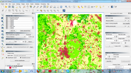
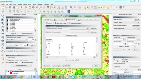
9. Perform maximum likelihood classification of the object segments using the Semiautomatic classification plugin: To open the plugin go to Raster --> Semi-Automatic Classification Plugin --> Semi-Automatic Classification Plugin. Click Show docks. In the Semi-Automatic:ROI creation window select input as 188_pca_indices_ pan_mean.tif., Select a training shapefile as train_segments_6class.shp. Leave the ROI parameters to default. In the Semi-Automatic: Classification window select classification algorithm to Maximum Likelihood, select qml as classification.qml. Check Create vector, Apply mask, Classification report and Calculate accuracy. Specify a cloud mask as cloud_mask.shp. Click Perform Classification and specify the output file as semi_automatic classification.shp. An additional output file semi_automatic classification.tif will be created. See Figure D. Import the classification style from classification.qml. To conduct an accuracy assessment for your map output, go to the Post processing tab and select Accuracy in the Semi-Automatic Classification Plugin window. Load semi_automatic_classification.tif in Select the classification to assess and train_segments_6class.shp in Select the reference shapefile and click Calculate error matrix (see figure E). We did all of this in ecercise 08. Shouldn't we just link there? - Levent (talk)

Figure C: Result of segmentation by mean shift clustering with the Orfeo Toolbox Mean Shift Segmentation algorithm	Figure D: Result of the semi-automatic maximum likelihood classification
Figure D: Error matrix for the semi-automatic maximum likelihood classification

Alternative supervised classification with Support Vector Machine (SVM)

1. Start Monteverdi.
2. Open 188_pca_indices_pan_mean.tif and train_segments_7class.shp in Monteverdi via File --> Open dataset.
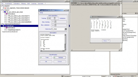
3. Go to Learning --> SVM classification (EXPERIMENTAL)
4. Load 188_pca_indices_pan_mean.tif as Input image and train_segments_7class.shp as Training/validation ROIs and press OK.
5. Specify the Class key as ID_class and click Train. A classification output is seen Monteverdi.
6. Click Validate to see classification accuracy and Calculate error matrix. See Figure G.

Supervised classification menu in Monteverdi with error matrix