Talk:Image classification

Article discussion

This section is meant solely for discussion purposes.
For a pre-version of the article, see #Article draft.

Article draft

Image classification covers a group of methods used to convert remotely sensed images in a manner that makes different thematic classes, e.g. forest, water or settlement areas, easier to recognize.

The basic concept is the identification of pixels with similar characteristics, and the aggregation of these pixels to classes. Of course, this assumed similarity has to be carefully defined. It is based on the spectral signature of the respective class, usually the combination of brightness values of the pixels on different bands. For a correct classification, ancillary data is needed to establish the different classes and their thematic meaning. This can be derived from ground information, or simply the researchers' knowledge of the terrain. The classification methods may be divided into unsupervised and supervised approaches. They are defined by the order in which the gathered information (spectral and ground based) is used.

The desired result of a classification is (1) a thematic map of the target area and (2) information on the accuracy of the map.

Unsupervised classification

Unsupervised classification is based on so called clustering algorithms, which assign pixels to classes by statistical means. The classes are not defined beforehand, they are established in the clustering process, hence the label unsupervised. After the algorithm finishes the job, the researcher has to label the output classes according to their thematic content.

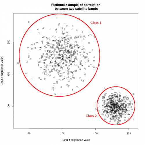
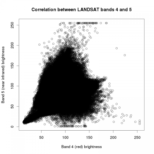
Clustering algorithms basically all work the same way: they compare the spectral similarity of pixels and, based on this information, aggregate them into groups. Imagine the brightness values of two sattelite bands, as shown in figure A. As you may know from the construction of color composites, objects on the earth's surface reflect differently in the different spectral intervals. E.g. vegetation may reflect strongly in the near infrared spectrum and little in the visible red spectrum. This leads to different correlations between the brightness values of different spectral bands of the same pixel. Thus, if brightness values are plotted against each other, more or less discrete groups become visible. These correlations make up the spectral signature of the pixels. In theory, the algorithm will recognize these signatures and aggregate the pixels accordingly. In practice, pixels rarely show such discrete spectral patterns (see figure B), which is why (1) more than two bands have to be used for classification and (2) the clustering process is subject to a more or less high error. Also, note that the spectral signature strongly depends on external factors, such as weather, atmospheric condition, human disturbance (farming, forest management...) or vegetation phenology (leaf production, flowering...).

A:Example plot of the brightness values of two satellite bands

B:Brightness values of LANDSAT bands 4 and 5

Iterative clustering

Iterative clustering, also known as migrating means requires a certain number of classes to be set beforehand. For every class, a point is set at a random position in the n-dimensional space (one dimension for each band, s.o.). Afterwards, each pixel value is assigned to the nearest point, so that classes are created. Then the mean of all classes are calculated and all pixels are assigned to the nearest mean. This procedure is repeated, until the overall distances of points to the respective means cannot be reduced anymore. All in all, this is an application of the least squares method also applied in linear regression analysis.

An example of three iterative clustering steps for two classes. Note that the steps are not limited to three, but carried out until the distance of points to class means is minimized.

Hierarchical clustering

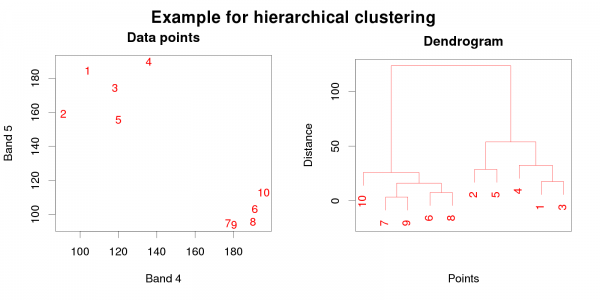
Hierarchical clustering algorithms start with the assumption that every pixel represents an own class. Then, with each iteration, pixels are assigned to the pixels nearest to them, thus creating a new class. The algorithm usually returns a data structure which can be visualized as a dendrogram (see figure A). If the dendrogram is read starting at the bottom, the aggregation of classes after each iteration can be retraced. Multiple classes at the bottom are aggregated into higher-ranking classes at the top (thus the label hierarchical). The researcher may decide which number of classes (i.e. which level of branches in the dendrogram) shall be used. This approach may be more accurate, as errors in the selection of the number of classes won't occur. Yet, as each pixel starts as a class of it's own, computation may take a long time for large data sets.

A: An illustration of hierarchical clustering. The left figure shows the data points, the right figure shows a dendrogram produced by hierarchical clustering. The two main branches can be interpreted as two classes, branches of higher order may be used if more classes are desired.