Approaches to populations of sample plots
Contents |
General observations
In forest inventory field sampling, the sampling elements that we select and observe are sample plots. Consequently, the population from which we sample is a population of sample plots.
Approach 1


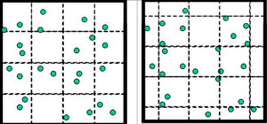
An intuitive approach is to imagine this population as the set of sample plots that covers the area of interest completely. This is depicted in Figure 1 for the two examples of square and hexagonal fixed area sample plots. The population consists of a discrete number of plots (see Figure 3, left). The sampling process is to select some of these plots. However, this approach does pose a series of interpretation and analysis problems; it works only for fixed area plots and within the class of fixed are plots only for some plot shapes. For the most frequently used circular plot, for example, this concept can not be applied.
Also, once the forest area of interest is defined (the area sampling frame), it is not clearly defined as well how the plots come to lie. Figure 2 shows one and the same population over which two different grids of plots are overlaid. In one case the square plots fit perfectly into the square area sampling frame, in the other case, there are various border plots with smaller size. The per-plot mean and variance will be different between the two sub-divisions; this is certainly an undesirable property of a population concept that the population parameters are not clearly defined. We conclude that this simple concept of populations of sample plots is not well suited as a model for forest inventory sampling.
Approach 2
The inclusion zone concept shows which bases on the idea to select points from the area sampling frame around which the sample trees are being selected along a defined plot design. This is a completely different view at the population of sample plots. It is some times called “the infinite population approach” because the population consists of the infinite number of points within the areal sampling frame. Each point possesses a characteristic which is being observed. However, that value is not being observed at the point itself, but it derives from the sample trees which are tallied around that sample point according to the rules that are defined by the plot design.
The inclusion zone concept and the infinite population approach belong together. Each tree k has its inclusion zone \(E_k\). While the size of this inclusion zone can be taken as a measure for the selection probability of that particular tree k, we may also follow a straightforward geometric interpretation that helps understanding the estimation, which is, in fact, based on unequal probability sampling (see also sampling with unequal selection probabilities).
If the tree k has an attribute value \(y_k\) (for example basal area in \(m^2\); or simply number of trees which is \(y_k=1\) for each tree, obviously) we imagine this value distributed evenly over the inclusion zone. Geometrically, that is a disk with the inclusion zone as base area \(a_k\) and a height which is defined by \(y_k\) as
\[d_k=\frac{y_k}{a_k}.\,\]
The value of \(d_k\) is constant over the entire inclusion zone and may be interpreted as density value. For the variable number of stems, \(d_k=1/a_k\), because \(y_k=1\).
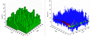
Fig 3. Illustration of approaches for plot populations for the same example population. Left: discrete population of square sample plots with defined positions. Right: each point in the area is a sampling element the value of which is determined by the surrounding trees (sample plot). Each point has a value which is here indicated through the cloud of points; in addition a trend surface is given.
The value of one sample element in the infinite population of sample points results from the sum of all such density values d which are present at the particular position x1i , x2i: . That defines eventually the infinite population of points which is indicated in Figure 70, right, as a cloud of points. The population total is then the integral over the entire area of all inclusion zones . Observe that this implies to integrate also outside the areal sampling frame of sample points where inclusion zones of border trees are outside the defined inventory area. This leads to the border correction issue which is dealt with in chapter 4.3.
From that infinite population, a sample of size n is selected. From a sample point i with the grid coordinates x1i, x2i the estimated total of forest area A derives from the Hansen-Hurwitz-estimator (this estimator is dealt with in chapter 5.9) from , where f() is the selection probability. Assuming independent random sampling, for all sample points. It follows . One may interpret this estimator also such that each observation yk is expanded with the plot-specific expansion factor EFk=A/ak.
From a sample of n randomly selected sample points, the total is eventually estimated as .
With this infinite population approach, most properties of plots and other issues in forest inventory sampling can be much better described (including the mirage technique for border plot correction) than with the discrete plot population approach.
References
- ↑ 1.0 1.1 1.2 Kleinn C. und F. Vilčko. 2005. Ein Vergleich von zwei methodischen Konzepten für die Grundgesamtheit von Probeflächen bei Waldinventuren. AFJZ 176(4):68-74.