Resource assessment exercises: nested fixed area plots

sorry:

This section is still under construction! This article was last modified on 07/23/2014. If you have comments please use the Discussion page or contribute to the article!

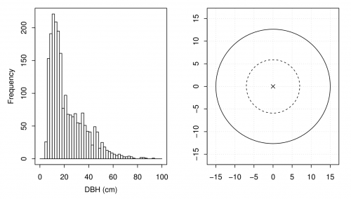
In the last subsection we saw that we “measured” 2,158 DBHs on the \(n=50\) fixed area plots. Many of the trees are relatively small, i.e., have small DBHs. Figure A shows a histogram of the variable dbh. The bin width is two centimeters.

bins <- seq(from=0, to=100, by=2) # define bin wiedth (here, 2 cm classes)
hist(fixed.area$dbh, breaks=bins, main="", xlab="DBH (cm)")

What the function seq() does

The function seq(from, to, by) creates a sequence of values. The argument by defines the step length. Alternatively you can use, e.g., length.out. For example seq(0, 1, length.out = 10)} creates a sequence from zero to one of length 10.

Figure A: Histogram of DBH in fixed.area and nested sample plot

We use the quantile() function to obtain a numerical representation of the DBH distribution.

quantile(fixed.area$dbh, probs=seq(from=0, to=1, by=0.1))

##   0%  10%  20%  30%  40%  50%  60%  70%  80%  90% 100% 
##    6    9   11   13   15   17   22   28   35   45   93

What the function quantile() does

The function quantile(x, ) provides sample quantiles for given probabilities (argument probs). The probabilities have lie between zero and one, i.e., [0, 1].

We see that many trees have a DBH below 15 cm. Measuring all the DBHs on a plot is often a tedious task. Moreover, small trees contribute relatively little to the BA ha\(^{-1}\). Can we reduce the number of small trees we need to measure?

In forest inventories nested plots are frequently used (see Figure A). Within the larger area (solid line) all trees with a DBH larger than 15 centimeters are measured, and small trees (\(\leq\)15 cm) are only recorded within the smaller circle (dashed line). The radius of the smaller plot is \(r_{\text{small}}=7.73\) and for the larger we still use a radius of \(r_{\text{large}}=15.45\).

We file MES.RData contains a data.frame named nested. The locations of the plots are exactly the same as for the fixed.area plots. However, we used a threshold diameter for small trees (\(\leq\)15 cm) in a nested plot design.

Here are the number of trees we measured.

## [1] 1624

## [1] 2158

Using the nested plot design we reduced the number of measured DBHs by 534. Does it reduce the precision of the BA ha\(^{-1}\) estimate considerably?

Firstly, we need to calculate the BA for each tree again. Secondly, we need to calculate the expansion factors for the larger and smaller nested plot.

## [1] 15.45

## [1] 7.725

## [1] 187.5

Thirdly, the BA per hectare and plot is calculated for the large and small plots and multiplied with the respective expansion factor.

Finally, we sum up the BA ha\(^{-1}\) for large and small plots.

The error message is printed because there are small plots that do not contain any trees, i.e., bal and bas do not have the same length. Here is a simple workaround.

Next, we compute the mean of the BA ha\(^{-1}\) per plot to estimate the population BA ha\(^{-1}\).

## [1] 34.62

Finally, we construct the confidence intervals around our estimated mean.

## [1] 3.245

## [1] 9.376

## [1] 6.522

## [1] 28.09

## [1] 41.14

Exercises

Repeat the tasks from the last exercise (Section [sub:fixedex]). Use the data in nested.Ex. Trees with a DBH \(\leq\) 15 cm have only been measured within a smaller circular plot with \(r=10\) meters.