Resource assessment exercises: nested fixed area plots

sorry:

This section is still under construction! This article was last modified on 07/23/2014. If you have comments please use the Discussion page or contribute to the article!

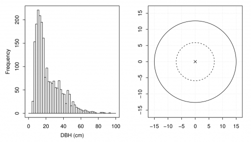
In the last subsection we saw that we “measured” 2,158 DBHs on the \(n=50\) fixed area plots. Many of the trees are relatively small, i.e., have small DBHs. Figure A shows a histogram of the variable dbh. The bin width is two centimeters.

bins <- seq(from=0, to=100, by=2) # define bin wiedth (here, 2 cm classes)
hist(fixed.area$dbh, breaks=bins, main="", xlab="DBH (cm)")

What the function seq() does

The function seq(from, to, by) creates a sequence of values. The argument by defines the step length. Alternatively you can use, e.g., length.out. For example seq(0, 1, length.out = 10)} creates a sequence from zero to one of length 10.

Figure A: Histogram of DBH in fixed.area and nested sample plot

We use the quantile() function to obtain a numerical representation of the DBH distribution.

quantile(fixed.area$dbh, probs=seq(from=0, to=1, by=0.1))

##   0%  10%  20%  30%  40%  50%  60%  70%  80%  90% 100% 
##    6    9   11   13   15   17   22   28   35   45   93

What the function quantile() does

The function quantile(x, ) provides sample quantiles for given probabilities (argument probs). The probabilities have lie between zero and one, i.e., [0, 1].

We see that many trees have a DBH below 15 cm. Measuring all the DBHs on a plot is often a tedious task. Moreover, small trees contribute relatively little to the BA ha\(^{-1}\). Can we reduce the number of small trees we need to measure?

In forest inventories nested plots are frequently used (see Figure [fig:hist]). Within the larger area (solid line) all trees with a DBH larger than 15 centimeters are measured, and small trees (\(\leq\)15 cm) are only recorded within the smaller circle (dashed line). The radius of the smaller plot is \(r_{\text{small}}=7.73\) and for the larger we still use a radius of \(r_{\text{large}}=15.45\).

We file MES.RData contains a data.frame named nested. The locations of the plots are exactly the same as for the fixed.area plots. However, we used a threshold diameter for small trees (\(\leq\)15 cm) in a nested plot design.

Here are the number of trees we measured.

## [1] 1624

## [1] 2158

Using the nested plot design we reduced the number of measured DBHs by 534. Does it reduce the precision of the BA ha\(^{-1}\) estimate considerably?

Firstly, we need to calculate the BA for each tree again. Secondly, we need to calculate the expansion factors for the larger and smaller nested plot.

## [1] 15.45

## [1] 7.725

## [1] 187.5

Thirdly, the BA per hectare and plot is calculated for the large and small plots and multiplied with the respective expansion factor.

Finally, we sum up the BA ha\(^{-1}\) for large and small plots.

'

The error message is printed because there are small plots that do not contain any trees, i.e., bal and bas do not have the same length. Here is a simple workaround.

Next, we compute the mean of the BA ha\(^{-1}\) per plot to estimate the population BA ha\(^{-1}\).

## [1] 34.62

Finally, we construct the confidence intervals around our estimated mean.

## [1] 3.245

## [1] 9.376

## [1] 6.522

## [1] 28.09

## [1] 41.14

Exercises

Repeat the tasks from the last exercise (Section [sub:fixedex]). Use the data in nested.Ex. Trees with a DBH \(\leq\) 15 cm have only been measured within a smaller circular plot with \(r=10\) meters.