Line sampling

Introduction

Line sampling uses one-dimensional lines as observation units, just as we may use for many purposes fixed area sample plots (two-dimensional observation units) or points (dimensionless observation units). Line sampling does here not refer to the so-called transects which usually mean elongated narrow strips, that is: two-dimensional plots. Depending on the dimensionality of the observation units, different types of observations can be made on them. There are three major uses of line sampling:

• It may be observed which portion of a sample line comes to lie in forest. These portions can be used to estimate the forest cover percent. This type of sampling is called line intercept sampling.

• It may be observed how many times a sample line intersects with a line feature in the landscape such as forest edges, roads or creeks. The number of intersections can be used to estimate the total length of these line features. This type of sampling is called line intersect sampling.

• It may be observed whether a population element is intersected or not by a sample line. By this, we may use the line samples to make a random selection of population elements in the absence of an a priori sampling frame.

A good reference for line sampling is deVries (1986) or earlier related studies by deVries.

Line intercept sampling

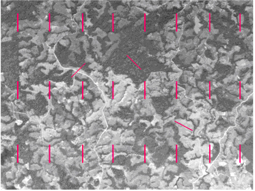
Line intercept sampling is used to estimate the cover of defined classes in the landscape, for example forest or forest types. Line samples are randomly placed over the area of interest and on each sample line it is observed which proportion comes to lie in the target area class. The observation per sample line can take on values between 0 and 1. From these observations, the mean, variance and error variance can be estimated along the known estimators. Line intercept sampling is typically applied in aerial photographs when rapid area estimations are desired. However it is also applied in the field: in large area forest inventory cluster sampling, one may use, for example, the connecting lines between sub-plots to do line intercept sampling. Figure 1 illustrates this approach by overlaying a systematic sample of equally oriented lines of n = 24 and a random sample of randomly located and randomly oriented lines of n = 3.

Figure 1. Application of line intercept sampling on an aerial photograph.

Let \(l_{i(in)}\) be the length of the sample line i which is inside the target condition class such as forest, \(l_{i(total)}\) be the total length of the sample line i; then, the observation \(y_i\) which is made on line i is

\[y_i = \frac {l_{i(in)}} {l_{i(total)}}\].

The estimated proportion \(\hat p\) in the region off interes is then estimated from n randomly placed sample lines from

\[\hat p=\frac {\sum_{i=1}^n y_i}{n}\]

and the variance in the population is estimated from

\[s^2=\frac {\sum_{i=1}^n (y_i - \hat p)^2}{n-1}\].

The error variance is <math>s_p^2 = \frac {s^2}{n}.