Introduction to resource assessment exercises
| sorry: |
This section is still under construction! This article was last modified on 05/10/2014. If you have comments please use the Discussion page or contribute to the article! |
- This article is part of the Resource assessment exercises. See the category page for a (chronological) table of contents.
Contents |
About this tutorial
The exercises are intended as supplementary material for the lecture Resource Assessments in Ecosystems (B.Sc. study program Molecular Ecosystem Sciences at the Georg—August University of Göttingen). Its main purpose is to demonstrate how to “translate” the formulas you have seen during the lectures into code. The main focus is, therefore, on coding, rather than on the underlying theory. Good introductory texts to the topics covered here include Cochran (1997) [1], Särndal et al. (1992) [2], Gregoire & Valentine (2008) [3], Robinson & Hamann (2011) [4] and in particular Kleinn (2003) [5]. Further information can be found all over the wiki and will be referenced accordingly.
Example data
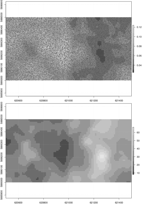
Throughout this document we will use a dataset that has been simulated in R. It is a “forest” covering an area of 50 hectares. There are two different forest types (or strata), each of size of 25 hectare. The two strata differ in how densely they are stocked (numbers of trees per hectare), the average diameter at breast height (DBH; measured at 1.3 meters above ground) and the distribution of DBHs. Figure A shows the spatial distribution of trees (top) and the spatial distribution of DBH values in the forest.

Since the dataset has been simulated we know the geographic position (\(x\)- and \(y\)-coordinates; EPSG code 32632), DBH (in centimeters), height (in meters) and species (either beech [Fagus sylvatica L.], or oak [Quercus robur L.]) of each tree.
The simulated data can be downloaded here (file trees.csv). The script that was used to generate the data can also be found there (file simulateForest.R).
Objectives
The simulated forest will serve as our “playground”. We will conduct several sample surveys in the “forest” using different response and sample designs. The sampled data will be analysed in R. We will assume that you are familiar with at least the basics of R. If not, you will find several useful tutorials and manuals on the (cran.r-project.org R website). Another good starting point is the Quick-R website.
At the end of each section you will find a couple of example questions. We highly recommend to work through these exercises. The file (exercises.RData) can also be found in the exercise data. The solutions to the exercises will be available soon.
Related articles
- Next article: Loading data
References
- ↑ Cochran, W.G., 1977. Sampling Techniques. John Wiley & Sons, New York, 3rd edition
- ↑ Särndal, C.-E., Swensson, B., Wretman, J., 1992. Model Assisted Survey Sampling. Second. ed, Springer Series in Statistics. Springer, New York.
- ↑ Gregoire, T.G., Valentine, H.T., 2008. Sampling Strategies for Natural Resources And The Environment, Applied Environmental Statistics. Chapman & Hall/CRC.
- ↑ Robinson, A.P., Hamann, J.D., 2011. Forest Analytics with R: an introduction. Springer, New York.
- ↑ Kleinn, C., 2013. Lecture Notes for the Teaching Module Forest Inventory.