Estimation on changes
| Line 96: | Line 96: | ||
If growth estimates are to be made from point relascope samples, all these elements of change need to be separately estimated. | If growth estimates are to be made from point relascope samples, all these elements of change need to be separately estimated. | ||
| + | |||
| + | ==Sampling with partial replacement== | ||
| + | |||
| + | [[File:6.1.4-fig107.png|right|thumb|300px|'''Figure 4''' | ||
| + | Plot combination schemes in sampling with partial replacement. (Kleinn 2007<ref name="kleinn2007">Kleinn, C. 2007. Lecture Notes for the Teaching Module Forest Inventory. Department of Forest Inventory and Remote Sensing. Faculty of Forest Science and Forest Ecology, Georg-August-Universität Göttingen. 164 S.</ref>).]] | ||
| + | When estimating only changes, then re-measured samples (permanent plots) are more cost-effective than temporary inventories. However, how can we be sure that at point 2 in time the sample (that had been defined at point 1 in time) has still the character of a statistical sample? To check that, one could opt to not establish all plots as permanent plots but only a part; installing at each point in time a set of temporary plots. This sampling strategy is called sampling with partial replacement (SPR) and has proven to be very efficient for both estimation of changes and also for the estimation of the status quo at point 2 in time. Sampling with partial replacement is schematically depicted in Figure 4. | ||
| + | The changes are estimated from the set of matched plots. The additional temporary plots at point 2 in time are being used to check whether the permanent plots are still “representative” for the stand; this can simple be done by performing, for example, a t-test checking whether the set of permanent plots and the set of temporary plots are statistically significantly different; if so, the hypothesis needs to be accepted that the two sets of plots do not come from the same population. This can happen, for example, if the permanent plots are marked such that they are visible for the forest manager. If then, the forest manager treats the permanent plots differently from the rest of the stand, it is clear that these differences will also be reflected in the comparison of the permanent and the temporary plots. | ||
| + | |||
| + | It is interesting to note, that SPR is also a very efficient technique to estimate the status quo at point 2 in time, because the information gathered at point 1 in time can be used as ancillary variable applying double sampling estimators, and one can assume that the correlation between the observations at point 1 in time and point 2 in time is high (which is one of the major preconditions for double sampling with the regression estimator to be efficient). | ||
==References== | ==References== | ||
Revision as of 20:27, 16 March 2011
| sorry: |
This section is still under construction! This article was last modified on 03/16/2011. If you have comments please use the Discussion page or contribute to the article! |
Contents |
General observations
In a “one-shot” forest inventory, the vast majority of measurements estimate the status quo for given attributes. However, estimation of changes is at least as important to evaluate the dynamics of the forest ecosystem and to monitor the silvicultural treatments and the performance of forest management.
There are only few change attributes that can be measured directly. Typical examples are increment borings, where the change (increment) of dbh over a certain period can directly be measured on a bore core and expanded to the entire cross section; and measurement of length of terminal shoots (or distances between whirls) for coniferous trees.
If repeated observations are made, estimation of change can be expressed as
\[change=c=\bar{y_2}-\bar{y_1},\,\]
where \(\bar{y_1}\) is the estimated mean at point 2 in time and \(\bar{y_1}\) is the estimated mean at point 1 in time. The estimated change is a linear combination of two random variables, i.e. the two estimated means can be considered random variables and they are “linked” by the linear operator “minus”. Then, the expected value and the variance of this linear combination can be determined along the rules presented in the context of stratification (there, however, weighted estimated means were added, while here, estimated means are subtracted); in stratification, the random variables (the stratum estimated results) were independent random variables, while in change estimation we deal either with dependent or with independent random variables:
- One may carry out an inventory in point 1 in time \(t_1\) and then another one independently of the first inventory in point 2 in time \(t_2\). Independent means here that at the two points in time different randomizations were done, and, therefore, different sample plots selected. The change is estimated then along \(c=\bar{y_2}-\bar{y_1}\), and the variance of the estimated change is the sum of the variances:
\[var(\bar{y_2}-\bar{y_1})=var\bar{y_1}+var{y_2}.\,\]
- However, one may at point 2 in time revisit the same plots that were established in point 1 in time. These plots are called “permanent sample plots” and their position needs to be recorded and marked such that they can be found after a certain time period. In that case, the estimated means are not independent, because in point 2 in time there was not an independent sample selection, but the same plots were used as in point 1 in time. Or put in other words: for each observation in point 2 in time, we can exactly assign a corresponding observation from point 1 in time (that is: the observations from the same plot). In that case, change c is also estimated from \(c=\bar{y_2}-\bar{y_1}\), but we need to take a covariance term in variance calculation into account:
\[var(\bar{y_2}-\bar{y_1}=var\bar{y_2}+var\bar{y_1}-2cov(y_1y_2).\,\]
As we are always interested in precise estimates, that is: low values for the variance, we may now wonder whether, given the same sample size in the two points in time, it is more recommendable to use dependent or independent inventories at the two points in time. The variances differ only in the covariance term. We may assume that the observations made on the same plot at different points in time are highly positively correlated (and have a high positive covariance). That means, in the case of dependent inventories (permanent plots) the covariance term is subtracted by the sum of the variances; leading to more precise estimates. This is actually conform with common sense considerations: in permanent inventories where the same plots are repeatedly observed, we can determine the differences (changes) for each plot – and not only for the entire population; we may, therefore, expect that this more detailed information leads also to more precise estimations of change.
Permanent plots


So-called permanent plots need to be installed when repeated observations of the same trees are to be made. While it is frequently said “we install permanent plots”, one will only see after the first re-measurement whether it is really permanent plots!
It is more costly to install plots that are to be used as permanent plots because:
- The plot location needs to be marked and or recorded such that it can be found again after some time (usually several years. This is done by determining the GPS coordinates and by drawing a draft of the way to the plot.
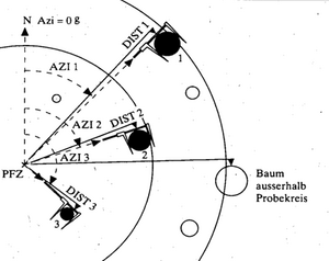
- The trees need to be mapped on the plot so that changes per individual tree can be observed. On circular plots that is done by measuring azimuth and distance of the trees to the plot center. On strip plots, the position of each tree is determined by the length measurement on the central line of the strip and by measuring the distance from the center line; in that case: do not forget to also record whether the tree is on the right or left side of the center line … This tree map is also very helpful in finding the sample plot at the second point in time.
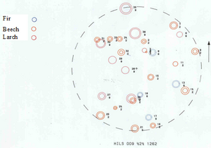
Figure 1 illustrates the position measurement of trees on a plot established as permanent plot. Here, dbh is measured with the caliper; in order to avoid that major discrepancies between the repeated measurements come from irregularities of the stem when different orientations of the caliper measurements at the two points in time were taken, in that inventory it was defined that all dbh measurements are to be taken such that the leg of the caliper points exactly to the plot center. Figure 2 illustrates a result plot map of re‑measured trees depicting the dbh of the trees and the change in dbh.
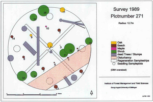
In some cases, it is not only of interest to map the tree positions but various other attributes as well like roads, dead wood, shrubs etc. This plot design is then called “mapped plot design”; it allows various more spatial type of analyses than spatially not explicit recording.
Permanent plots are actually one of the backbones of forest management and yield regulation, because they allow us to learn a lot about forest growth and productivity. To install a network of permanent plots, however, is a high investment at the establishment point in time – and it requires a permanent infrastructure for the re-measurements: the data need to be stored and maintained in an information system; and at the later points in time when re-measurements are to be taken, it must not only be known where the plots are but also where the data are. While this sounds somewhat unnecessary to mention – it is probably one of the major practical problems of permanent plots.
Permanent plot designs must be planned with care in order to produce meaningful information. It may be interesting to note that it was actually the question of harmonization and standardization of permanent plots and data from permanent plots that lead more than 100 years ago to the founding of the International Union of Forest Research Organizations (IUFRO); thus, the goal to provide comparable and high quality (international) forest and tree data is old.
High investments and long term commitment go along with permanent plots. The real value of permanent plots may show after several years (or even decades) only.
Growth components
While the assessment and analysis of forest growth is another discipline in the forest sciences than forest inventory, we address here some issues. The difference
\[\bar{V_2}-\bar{V_1}\,\]
that we observe from two repeated measurements is actually not the growth but incorporates various growth components. The difference results from
\[V_2-V_1=S+I-M-C\,\],
where
\(V_1\,\) \(=\) volume at t2; \(V_2\,\) \(=\,\) volume at t1; \(S\,\) \(=\,\) survivor growth; \(I\,\) \(=\,\) ingrowths; \(M\,\) \(=\,\) mortality; \(C\,\) \(=\,\) cut.
For a comprehensive analysis of volume change and in order to estimate growth, all components must be estimated from the repeated observations (permanent plots). It can be carried out most easily from fixed area plots along the equation given above. There, we have only one type of ingrowth, which is the trees which grow beyond the minimum dbh.
It is slightly more complex from point‑relascope samples, because, in addition to the ingrowth trees (that are only counted in point 2 in time but were also in-trees at point 1 in time but
below the minimum diameter), we also have the ongrowth trees and the nongrowth trees:
- Survivor trees are merchantable-and-in at both points in time
- Ingrowth trees are sub-merchantable-and-in at time 1 and merchantable at time 2
- Ongrowth trees are sub-merchantable-and-out at time 1 but merchantable-and-in at time 2
- Nongrowth trees are merchantable-and-out at time 1 but merchantable-and-in at time 2
- Cut trees are merchantable-and-in at time 1 but cut prior to time 2
- Mortality trees are merchantable-and-in at time 1 but dead prior to time 2.
If growth estimates are to be made from point relascope samples, all these elements of change need to be separately estimated.
Sampling with partial replacement

When estimating only changes, then re-measured samples (permanent plots) are more cost-effective than temporary inventories. However, how can we be sure that at point 2 in time the sample (that had been defined at point 1 in time) has still the character of a statistical sample? To check that, one could opt to not establish all plots as permanent plots but only a part; installing at each point in time a set of temporary plots. This sampling strategy is called sampling with partial replacement (SPR) and has proven to be very efficient for both estimation of changes and also for the estimation of the status quo at point 2 in time. Sampling with partial replacement is schematically depicted in Figure 4. The changes are estimated from the set of matched plots. The additional temporary plots at point 2 in time are being used to check whether the permanent plots are still “representative” for the stand; this can simple be done by performing, for example, a t-test checking whether the set of permanent plots and the set of temporary plots are statistically significantly different; if so, the hypothesis needs to be accepted that the two sets of plots do not come from the same population. This can happen, for example, if the permanent plots are marked such that they are visible for the forest manager. If then, the forest manager treats the permanent plots differently from the rest of the stand, it is clear that these differences will also be reflected in the comparison of the permanent and the temporary plots.
It is interesting to note, that SPR is also a very efficient technique to estimate the status quo at point 2 in time, because the information gathered at point 1 in time can be used as ancillary variable applying double sampling estimators, and one can assume that the correlation between the observations at point 1 in time and point 2 in time is high (which is one of the major preconditions for double sampling with the regression estimator to be efficient).
References
- ↑ 1.0 1.1 1.2 Brändli U.B., A. Herold, H. Stierlin und J. Zinggeler 1994. Schweizerisches Landesforst-inventar. Anleitung für die Feldaufnahmen der Erhebung 1993-1995. Birmensdorf, Eidg. Forschungsanstalt für Wald, Schnee und Landschaft. 204 S.
- ↑ Kleinn, C. 2007. Lecture Notes for the Teaching Module Forest Inventory. Department of Forest Inventory and Remote Sensing. Faculty of Forest Science and Forest Ecology, Georg-August-Universität Göttingen. 164 S.