Pair difference technique example
(→Example 1) |
|||
| Line 8: | Line 8: | ||
Taking a systematic sample of <math>n=10</math> elements, there are not many possibilities in our small example population. In fact, if the there shall be an equal distance between the elements in the list, this distance must be <math>30/10=3</math>. Then, there are only three possible systematic samples having element 1, 2, or 3 as starting elements and then taking every third element. These three samples are listed and analyzed in Table 1. | Taking a systematic sample of <math>n=10</math> elements, there are not many possibilities in our small example population. In fact, if the there shall be an equal distance between the elements in the list, this distance must be <math>30/10=3</math>. Then, there are only three possible systematic samples having element 1, 2, or 3 as starting elements and then taking every third element. These three samples are listed and analyzed in Table 1. | ||
| + | |||
[[File:5.5.6.4-tab19.png|center|thumb|400px|'''Table 1''' The population of all possible systematic samples of size <math>n=10</math> drawn from the example population. There are only 3 possibilities. PD-5 and 9 are the estimated error variances from the pair differences method with 5 non-overlapping and 9 overlapping pairs of sampled values.]] | [[File:5.5.6.4-tab19.png|center|thumb|400px|'''Table 1''' The population of all possible systematic samples of size <math>n=10</math> drawn from the example population. There are only 3 possibilities. PD-5 and 9 are the estimated error variances from the pair differences method with 5 non-overlapping and 9 overlapping pairs of sampled values.]] | ||
As these three samples are the entire population of all possible samples of size 10 taken systematically (that is: equidistantly from the population listing) we can calculate here the expected value of the applied estimators directly. | As these three samples are the entire population of all possible samples of size 10 taken systematically (that is: equidistantly from the population listing) we can calculate here the expected value of the applied estimators directly. | ||
| + | |||
In Table 1, the estimators of simple random sampling were applied to the three samples producing the estimations of the mean and variance. We see that the expected value of the estimated mean is equal to the population value so that we can assume that that estimator is unbiased. However, the expected value of the estimated variance is higher than the true population variance which indicates in an empirical manner that the simple random sampling variance estimator is biased for systematic sampling. | In Table 1, the estimators of simple random sampling were applied to the three samples producing the estimations of the mean and variance. We see that the expected value of the estimated mean is equal to the population value so that we can assume that that estimator is unbiased. However, the expected value of the estimated variance is higher than the true population variance which indicates in an empirical manner that the simple random sampling variance estimator is biased for systematic sampling. | ||
| Line 30: | Line 32: | ||
where the pairs had been built from neighboring values in the population list. | where the pairs had been built from neighboring values in the population list. | ||
| + | |||
| + | {{SEO | ||
| + | |keywords=pair difference technique,variance issue,systematic sampling | ||
| + | |descrip=The pair difference technique is a method to calculate the error variance in systematic sampling. | ||
| + | }} | ||
==References== | ==References== | ||
Revision as of 16:08, 8 February 2011
Example 1
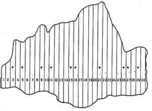
Systematic sampling from the example population in Figure 1 (Klein 2007[1]).

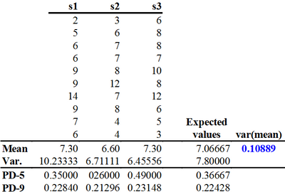
Taking a systematic sample of \(n=10\) elements, there are not many possibilities in our small example population. In fact, if the there shall be an equal distance between the elements in the list, this distance must be \(30/10=3\). Then, there are only three possible systematic samples having element 1, 2, or 3 as starting elements and then taking every third element. These three samples are listed and analyzed in Table 1.
As these three samples are the entire population of all possible samples of size 10 taken systematically (that is: equidistantly from the population listing) we can calculate here the expected value of the applied estimators directly.
In Table 1, the estimators of simple random sampling were applied to the three samples producing the estimations of the mean and variance. We see that the expected value of the estimated mean is equal to the population value so that we can assume that that estimator is unbiased. However, the expected value of the estimated variance is higher than the true population variance which indicates in an empirical manner that the simple random sampling variance estimator is biased for systematic sampling.
The parametric error variance can be calculated as the variance from the population of all estimated means. In this case
\(var(\bar y)=0.10889\,\),
which is only about one fifth of the error variance for simple random sampling with the same sample size! If we estimated the error variance of the estimated mean with the simple random sampling estimator we would produce, as expected, a considerable over-estimation (conservative estimation)\[var(\bar y)=\frac{7.8}{10}=0.78\,\].
Application of the pair differences technique has also been calculated for each of the three systematic samples. The estimations are given in the last two lines in Table 1.
Two options were applied:
- With 5 non-overlapping pairs of observations and
- With 9 overlapping pairs;
where the pairs had been built from neighboring values in the population list.
References
- ↑ Kleinn, C. 2007. Lecture Notes for the Teaching Module Forest Inventory. Department of Forest Inventory and Remote Sensing. Faculty of Forest Science and Forest Ecology, Georg-August-Universität Göttingen. 164 S.
- ↑ de Vries, P.G., 1986. Sampling Theory for Forest Inventory. A Teach-Yourself Course. Springer. 399 p.
