Talk:Image classification
(→Maximum likelihood classifier) |
(→Maximum likelihood classifier) |
||
| (17 intermediate revisions by one user not shown) | |||
| Line 150: | Line 150: | ||
======Maximum likelihood classifier====== | ======Maximum likelihood classifier====== | ||
The maximum likelihood classifier ist based on methods | The maximum likelihood classifier ist based on methods | ||
| − | of [[:wikipedia:Bayesian statistics|Bayesian statistics]]. | + | of [[:wikipedia:Bayesian statistics|Bayesian statistics]]. We |
| − | + | cannot provide the basics of this subject here, but | |
| + | see the [[#External links|external links]] section for a short tutorial on bayesian statistics. | ||
The maximum likelihood | The maximum likelihood | ||
classifier calculates the ''likelihood'' | classifier calculates the ''likelihood'' | ||
with which a pixel belongs to each class, | with which a pixel belongs to each class, | ||
and assigns it to the class for which the likelihood is highest. | and assigns it to the class for which the likelihood is highest. | ||
| + | The likelihood estimation is based on ''bayes' theorem'', | ||
| + | which estimates the likelihood of an event <math>A</math> | ||
| + | occuring given a certain condition <math>B</math>: | ||
| + | |||
| + | :<math>P(A|B) = P(B|A) \frac{P(A)}{P(B)}</math> | ||
| + | |||
| + | Here, <math>P(A|B)</math> ist the probability of event | ||
| + | <math>A</math> occuring if condition <math>B</math> | ||
| + | is given, also called the ''conditional probability''. | ||
| + | <math>P(A)</math> is called the ''prior'' | ||
| + | probability of the event <math>A</math>, i.e. the | ||
| + | probability for <math>A</math> without condition | ||
| + | <math>B</math> given. Vice versa, <math>P(B|A)</math> ist | ||
| + | the probability of condition <math>B</math> being | ||
| + | given and <math>A</math> occuring at the same time, | ||
| + | and <math>P(B)</math> ist the probability of condition | ||
| + | <math>B</math> occuring at all, again called the | ||
| + | ''prior'' probability. | ||
| + | |||
| + | In bayesian classification, the bayesian theorem is | ||
| + | put to use to estimate the likelihood of a pixel | ||
| + | with a spectral signature <math>x_i</math> belonging | ||
| + | to a class <math>w_j</math> <ref name=mather10>Mather, P. & Tso, B. Classification Methods for Remotely Sensed Data, Second Edition. (CRC Press, 2010).</ref>: | ||
| + | |||
| + | :<math> P(w_j|x_i) = P(x_j|w_j) \frac{P(w_j)}{P(x_i)} </math> | ||
| + | |||
| + | The spectral signatures of the pixels <math>x</math> are generally assumed to be uniformely | ||
| + | distributed, i.e. when picking one pixel at random, each spectral signature has the | ||
| + | same probability to occur. Note that this assumption will always be violated to | ||
| + | some degree in real life. Assuming the uniform distribution of spectral | ||
| + | signatures, the above equation can be rewritten to: | ||
| + | |||
| + | :<math> P(w_j|x_i) \propto P(x_j|w_j) P(w_j) </math> | ||
| + | |||
| + | meaning that the likelihood of a pixel with spectral signature | ||
| + | <math>x_i</math> belonging to a class <math>w_j</math> | ||
| + | is proportional to the product of the conditional | ||
| + | probability of the spectral signature and the prior | ||
| + | probability of the class. | ||
| + | Based on this equation, the criterion on which the | ||
| + | classifier is based can be expressed as: | ||
| + | |||
| + | :<math> w_k = \forall w_j\, arg\,max\{P(x_j|w_j) P(w_j)\} </math> | ||
| + | <!-- In Mather & Tso, the "for all" term is set right in the middle | ||
| + | under "arg max", but I don't know how to code this in wiki | ||
| + | math-syntax right now (Levent) --> | ||
| − | + | This means that a pixel is | |
| − | + | assigned to the class <math>w_k</math> for which the | |
| + | likelihood of the spectral signature to occur is | ||
| + | highest (denoted by <math>arg\,max</math>). | ||
| + | For this, the likelihoods for all classes have to | ||
| + | be computed (denoted by <math>\forall w_j</math>). | ||
====Generalization stage==== | ====Generalization stage==== | ||
Latest revision as of 07:54, 11 October 2013
Contents |
[edit] Article discussion
- This section is meant solely for discussion purposes.
For a pre-version of the article, see #Article draft.
- This section is meant solely for discussion purposes.
[edit] Article draft
Image classification covers a group of methods used to convert remotely sensed images in a manner that makes different thematic classes, e.g. forest, water or settlement areas, easier to recognize.
The basic concept is the identification of pixels with similar characteristics, and the aggregation of these pixels to classes. Of course, this assumed similarity has to be carefully defined. It is based on the spectral signature of the respective class, usually the combination of brightness values of the pixels on different bands. For a correct classification, ancillary data is needed to establish the different classes and their thematic meaning. This can be derived from ground information, or simply the researchers' knowledge of the terrain. The classification methods may be divided into unsupervised and supervised approaches. They are defined by the order in which the gathered information (spectral and ground based) is used.
The desired result of a classification is (1) a thematic map of the target area and (2) information on the accuracy of the map. [1]
[edit] Unsupervised classification
Unsupervised classification is based on so called clustering algorithms, which assign pixels to classes by statistical means. The classes are not defined beforehand, they are established in the clustering process, hence the label unsupervised. After the algorithm finishes the job, the researcher has to label the output classes according to their thematic content.
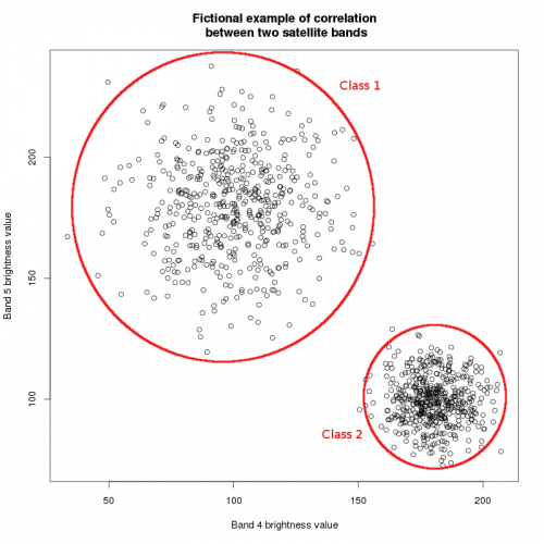
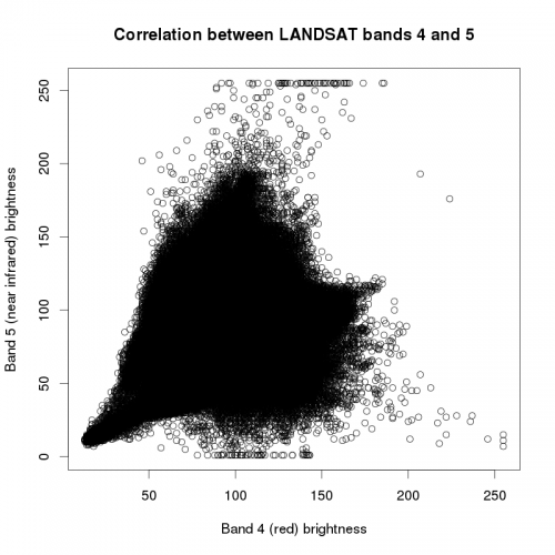
Clustering algorithms basically all work the same way: they compare the spectral similarity of pixels and, based on this information, aggregate them into groups. Imagine the brightness values of two sattelite bands, as shown in figure A. As you may know from the construction of color composites, objects on the earth's surface reflect differently in the different spectral intervals. E.g. vegetation may reflect strongly in the near infrared spectrum and little in the visible red spectrum. This leads to different correlations between the brightness values of different spectral bands of the same pixel. Thus, if brightness values are plotted against each other, more or less discrete groups become visible. These correlations make up the spectral signature of the pixels. In theory, the algorithm will recognize these signatures and aggregate the pixels accordingly. In practice, pixels rarely show such discrete spectral patterns (see figure B), which is why (1) more than two bands have to be used for classification and (2) the clustering process is subject to a more or less high error. Also, note that the spectral signature strongly depends on external factors, such as weather, atmospheric condition, human disturbance (farming, forest management...) or vegetation phenology (leaf production, flowering...). The most commonly used methods for unsupervised classification are iterative and hierarchical clustering.
[edit] Iterative clustering
Iterative clustering, also known as migrating means requires a certain number of classes to be set beforehand. For every class, a point is set at a random position in the n-dimensional space (one dimension for each band, s.o.). Afterwards, each pixel value is assigned to the nearest point, so that classes are created. The euclidean distance between a point \(x\) and mean of class \(i\) is calculated with the following equation, where \(x_i\) is the pixel and \(\mu_k\) is the mean for the respective sattelite band \(k\), the total number of bands being \(n\)\[ d_{E_i}=\sqrt{\sum\limits_{k=1}^n (x_i - \mu_k)^2} \]
Then the means of all classes are calculated and all pixels are assigned to the nearest mean. This procedure is repeated, until the overall distances of points to the respective means cannot be reduced anymore. Based on the above equation, the distance of all pixels to it's class mean is minimized\[ d_E=\sum\limits_{i=1}^m \sqrt{\sum\limits_{k=1}^n (x_i - \mu_k)^2} = \sum\limits_{i=1}^n d_{E_i} = min \]
All in all, this is an application of the least squares method also applied in linear regression analysis.
[edit] Hierarchical clustering
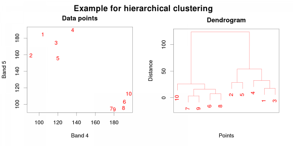
Hierarchical clustering algorithms start with the assumption that every pixel represents an own class. Then, with each iteration, pixels are assigned to the pixels nearest to them, thus creating a new class. The algorithm usually returns a data structure which can be visualized as a dendrogram (see figure A). If the dendrogram is read starting at the bottom, the aggregation of classes after each iteration can be retraced. Multiple classes at the bottom are aggregated into higher-ranking classes at the top (thus the label hierarchical). The researcher may decide which number of classes (i.e. which level of branches in the dendrogram) shall be used. This approach may be more accurate, as errors in the selection of the number of classes won't occur. Yet, as each pixel starts as a class of it's own, computation may take a long time for large data sets.
[edit] Supervised classification
As mentioned in the introduction, the methodical steps of supervised classification are conducted in the opposite order to unsupervised classification. While in unsupervised classification, the thematic classes are assigned to the spectral classes after the latter are created, in the supervised classification process, the thematic classes are set beforehand.
According to Wilkie & Finn[1], for supervised classification to be effective, we must be able to:
- Generate a classification that can assign at best every pixel to a class
- Detect and delete outliers (pixels which don't belong to any given class)
- Extract the spectral signature from a sample of pixels representing one class
- Identify the bands that can be aggregated to a group with highest possible between-group distance
- Select the most appropriate classifier for the available data/image size
- Assess the accuracy of the classification
The usual operational procedure works like this:
[edit] Training stage
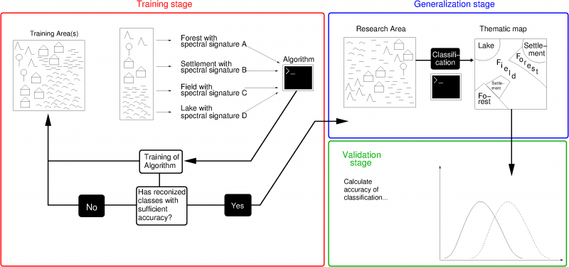
The spectral signatures are derived from one or more training areas. These are areas with classes already known to the researcher. They may have been derived by a preceding unsupervised classification, field observations, existing maps, interpretation of aerial photography or a combination of several methods. The selection of training areas is the most important step of the classification routine, as the extracted spectral signatures will determine the classification accuracy[1]. Based on the derived spatial signatures, a classification algorithm is "trained", i.e. configured in a manner that enables it to classify a target area with maximum accuracy. There are several types of algorithms, which are called classifiers.
[edit] Classifiers
[edit] Box classifier
The box classifier is a quite straightforward way to assign pixels to the given landscape classes. Only the minimum and maximum of the brightness value of each spectral band has to be defined for each class. In the two-dimensional space, the minima and maxima construct a "box", hence the name. The classifier is easy to implement, but provides no reasonable way of assigning pixels which lie in intersecting boxes.
[edit] Minimum distance classifier
The minimum distance classifier works just like the final stage of the iterative clustering algorithm in unsupervised classification. Here, as the spectral signatures of each class are already known, the means for each landscape classes spectral values are set beforehand. Each pixel is assigned to the class mean to which it lies in the shortes euclidean distance. The advantage of this classifier lies in it's mathematical and compultational simplicity. Yet, it is insensitive to different degrees of variance in the data, which increases the risk of misclassificatin if pixels' spectral signatures lie close to each other.
[edit] Maximum likelihood classifier
The maximum likelihood classifier ist based on methods of Bayesian statistics. We cannot provide the basics of this subject here, but see the external links section for a short tutorial on bayesian statistics. The maximum likelihood classifier calculates the likelihood with which a pixel belongs to each class, and assigns it to the class for which the likelihood is highest. The likelihood estimation is based on bayes' theorem, which estimates the likelihood of an event \(A\) occuring given a certain condition \(B\):
\[P(A|B) = P(B|A) \frac{P(A)}{P(B)}\]
Here, \(P(A|B)\) ist the probability of event \(A\) occuring if condition \(B\) is given, also called the conditional probability. \(P(A)\) is called the prior probability of the event \(A\), i.e. the probability for \(A\) without condition \(B\) given. Vice versa, \(P(B|A)\) ist the probability of condition \(B\) being given and \(A\) occuring at the same time, and \(P(B)\) ist the probability of condition \(B\) occuring at all, again called the prior probability.
In bayesian classification, the bayesian theorem is put to use to estimate the likelihood of a pixel with a spectral signature \(x_i\) belonging to a class \(w_j\) [2]:
\[ P(w_j|x_i) = P(x_j|w_j) \frac{P(w_j)}{P(x_i)} \]
The spectral signatures of the pixels \(x\) are generally assumed to be uniformely distributed, i.e. when picking one pixel at random, each spectral signature has the same probability to occur. Note that this assumption will always be violated to some degree in real life. Assuming the uniform distribution of spectral signatures, the above equation can be rewritten to:
\[ P(w_j|x_i) \propto P(x_j|w_j) P(w_j) \]
meaning that the likelihood of a pixel with spectral signature \(x_i\) belonging to a class \(w_j\) is proportional to the product of the conditional probability of the spectral signature and the prior probability of the class. Based on this equation, the criterion on which the classifier is based can be expressed as:
\[ w_k = \forall w_j\, arg\,max\{P(x_j|w_j) P(w_j)\} \]
This means that a pixel is assigned to the class \(w_k\) for which the likelihood of the spectral signature to occur is highest (denoted by \(arg\,max\)). For this, the likelihoods for all classes have to be computed (denoted by \(\forall w_j\)).
[edit] Generalization stage
After the algorithm has been sufficiently trained, it can be applied to raster data of the respective research areas. It processes each pixel of the map separately, assigning it to one of the predefined classes, or classifying it as an outlier.
[edit] Validation stage
After the imagery of interest has been classified, the results need to be thoroughly validated. Image classifications generated by any method are always subject to a certain degree of error. This error needs to be assessed, which can be done by several means of accuracy assessment.
[edit] Advantages and limits to supervised classification
An advantage of supervised classification algorithms is their pixel based way of processing. Whereas unsupervised methods need to aggregate pixels into groups, always processing several pixels at a time, supervised algorithms simply assign each single pixel to a class, based on it's spectral signature.
On the other hand, developing a new classification is time consuming. This is why in practice, already tried and tested systems are used and modified if necessary. Locally developed systems, which may be used only once, do not provide the possibility of comparing results to other studies or sharing data [1].
[edit] Image classification in forestry
[edit] Related articles
[edit] References
- ↑ 1.0 1.1 1.2 1.3 Wilkie, D. S. Remote sensing imagery for natural resources monitoring: a guide for first-time users. (Columbia Univ. Press, c1996).
- ↑ Mather, P. & Tso, B. Classification Methods for Remotely Sensed Data, Second Edition. (CRC Press, 2010).
[edit] External links
- Homepage of Kevin Boone, with an easy to understand tutorial on Bayesian statistics.


