Fixed area plots at the stand boundary
| (11 intermediate revisions by 2 users not shown) | |||
| Line 1: | Line 1: | ||
| − | {{ | + | {{Ficontent}} |
| − | + | ==The mirage technique== | |
| − | + | ||
| − | [[ | + | [[Fixed area plots]] are selected via their centers: if a sample point falls into [[Forest Definition|forest]], then a plot is established. For all sample points that may fall outside the forest area, no plot is established. It may happen that the sample point comes to lie close to the [[Forest Boundary|forest boundary]] so that part of the sample plot slops over. Of course, if this is not taken into account, an error is induced because the [[Tree Definition|tree]] observations that are made refer to a smaller [[plot area]] only. |
| − | [[File:4.3-fig56.png|center|thumb| | + | [[File:4.3-fig56.png|center|thumb|350px|'''Figure 1''' Different techniques applied to boundary plots. Only the mirage technique is not causing a systematic error. From left to right: mirage method, shifting the plot, enlarging the circular plot at the same location such that the plot area is maintained, and disregarding the slop-over part of the plot (Kleinn 2007<ref name="kleinn2007">Kleinn, C. 2007. Lecture Notes for the Teaching Module Forest Inventory. Department of Forest Inventory and Remote Sensing. Faculty of Forest Science and Forest Ecology, Georg-August-Universität Göttingen. 164 S.</ref>).]] |
| − | + | To correct for this effect, various techniques are applied in practice, as depicted in Figure 1. The mirage technique is recommended and commonly applied; it is simple to do and does not produce a systematic error. [[Plot shifting]] is – from a strict statistical point of view – never permitted. Using option D in Figure 1, one needs to take into account that plots have different areas; then, the [[ratio estimator]] may be applied which complicated the estimation process a little bit. | |
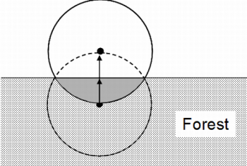
| − | + | [[File:4.3-fig57.png|center|thumb|350px|'''Figure 2''' Principle of the mirage method for border plot correction. The center of the plot is mirrored at the forest edge outside the forest. From that new point, again a circular plot is laid out and all trees tallied again which fall into it; these trees are observed twice (Kleinn 2007<ref name="kleinn2007">Kleinn, C. 2007. Lecture Notes for the Teaching Module Forest Inventory. Department of Forest Inventory and Remote Sensing. Faculty of Forest Science and Forest Ecology, Georg-August-Universität Göttingen. 164 S.</ref>).]] | |
The mirage technique is easily applied as illustrated in Figure 2: the center of a border plot is mirrored at the stand boundary outside the forest. From this mirrored sample point, the plot is again laid out. Most of that plot is outside the forest, but those trees that are in this plot are tallied again. That means that some trees at the stand boundary are recorded twice and count twice for the plot observation. | The mirage technique is easily applied as illustrated in Figure 2: the center of a border plot is mirrored at the stand boundary outside the forest. From this mirrored sample point, the plot is again laid out. Most of that plot is outside the forest, but those trees that are in this plot are tallied again. That means that some trees at the stand boundary are recorded twice and count twice for the plot observation. | ||
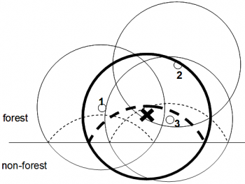
While the mirage procedure may sound strange at the first glance, the mathematical proof can easily be given applying the [[Fixed area plots#The inclusion zone concept|inclusion zone]] approach. This is illustrated in Figure 3: there are three trees close to the stand boundary. Two are so close that part of their inclusion zone is outside the forest. As, per definition, sample points can not be selected outside the forest, these trees 1 and 3 have parts of their inclusion zones that can not be sampled (if not properly corrected for); their selection probability would be corresponding to the area of the inclusion zone that is inside the forest stand; that is: the selection probability of the trees close to the stand boundary would be smaller. | While the mirage procedure may sound strange at the first glance, the mathematical proof can easily be given applying the [[Fixed area plots#The inclusion zone concept|inclusion zone]] approach. This is illustrated in Figure 3: there are three trees close to the stand boundary. Two are so close that part of their inclusion zone is outside the forest. As, per definition, sample points can not be selected outside the forest, these trees 1 and 3 have parts of their inclusion zones that can not be sampled (if not properly corrected for); their selection probability would be corresponding to the area of the inclusion zone that is inside the forest stand; that is: the selection probability of the trees close to the stand boundary would be smaller. | ||
| − | [[File:4.3- | + | [[File:4.3-fig58.png|center|thumb|350px|'''Figure 3''' Illustration of the inclusion zone approach at the stand boundary, and application of the mirage technique. The mirage technique guarantees that those parts of the inclusion zones that are outside the forest and that would have a probability of 0 to be sampled are properly taken into account (Kleinn an Vilcko 2005<ref name="kleinn_vilcko2005">Kleinn C. und F. Vilčko. 2005. Ein Vergleich von zwei methodischen Konzepten für die Grundgesamtheit von Probeflächen bei Waldinventuren. AFJZ 176(4):68-74.</ref>).]] |
| − | This is certainly not acceptable under the assumption of equal selection probabilities that we usually apply when [[Simple random sampling|randomly sampling]]. In order to correct for this systematic reduction of selection probability we mirror the inclusion zones back into the forest stand. Then the entire inclusion zone is within the area that can theoretically have a sample point. If a sample point falls then into an area where the inclusion zone of a border tree is folded back, this tree, of course, needs to be tallied twice. In effect, this is exactly what the mirage technique is doing: tallying all those trees twice whose inclusion zones are folded back into the stand where the sample point comes to lie. | + | This is certainly not acceptable under the assumption of equal selection probabilities that we usually apply when [[Simple random sampling|randomly sampling]]. In order to correct for this systematic reduction of selection probability we mirror the inclusion zones back into the forest stand. Then the entire inclusion zone is within the area that can theoretically have a sample point. If a sample point falls then into an area where the inclusion zone of a border tree is folded back, this tree, of course, needs to be tallied twice. In effect, this is exactly what the mirage technique is doing: tallying all those trees twice whose inclusion zones are folded back into the stand where the sample point comes to lie. |
| + | |||
| + | ==References== | ||
| + | <references/> | ||
{{SEO | {{SEO | ||
Latest revision as of 10:57, 28 October 2013
[edit] The mirage technique
Fixed area plots are selected via their centers: if a sample point falls into forest, then a plot is established. For all sample points that may fall outside the forest area, no plot is established. It may happen that the sample point comes to lie close to the forest boundary so that part of the sample plot slops over. Of course, if this is not taken into account, an error is induced because the tree observations that are made refer to a smaller plot area only.

To correct for this effect, various techniques are applied in practice, as depicted in Figure 1. The mirage technique is recommended and commonly applied; it is simple to do and does not produce a systematic error. Plot shifting is – from a strict statistical point of view – never permitted. Using option D in Figure 1, one needs to take into account that plots have different areas; then, the ratio estimator may be applied which complicated the estimation process a little bit.

The mirage technique is easily applied as illustrated in Figure 2: the center of a border plot is mirrored at the stand boundary outside the forest. From this mirrored sample point, the plot is again laid out. Most of that plot is outside the forest, but those trees that are in this plot are tallied again. That means that some trees at the stand boundary are recorded twice and count twice for the plot observation. While the mirage procedure may sound strange at the first glance, the mathematical proof can easily be given applying the inclusion zone approach. This is illustrated in Figure 3: there are three trees close to the stand boundary. Two are so close that part of their inclusion zone is outside the forest. As, per definition, sample points can not be selected outside the forest, these trees 1 and 3 have parts of their inclusion zones that can not be sampled (if not properly corrected for); their selection probability would be corresponding to the area of the inclusion zone that is inside the forest stand; that is: the selection probability of the trees close to the stand boundary would be smaller.

This is certainly not acceptable under the assumption of equal selection probabilities that we usually apply when randomly sampling. In order to correct for this systematic reduction of selection probability we mirror the inclusion zones back into the forest stand. Then the entire inclusion zone is within the area that can theoretically have a sample point. If a sample point falls then into an area where the inclusion zone of a border tree is folded back, this tree, of course, needs to be tallied twice. In effect, this is exactly what the mirage technique is doing: tallying all those trees twice whose inclusion zones are folded back into the stand where the sample point comes to lie.
[edit] References
- ↑ 1.0 1.1 Kleinn, C. 2007. Lecture Notes for the Teaching Module Forest Inventory. Department of Forest Inventory and Remote Sensing. Faculty of Forest Science and Forest Ecology, Georg-August-Universität Göttingen. 164 S.
- ↑ Kleinn C. und F. Vilčko. 2005. Ein Vergleich von zwei methodischen Konzepten für die Grundgesamtheit von Probeflächen bei Waldinventuren. AFJZ 176(4):68-74.