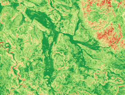
Digital Elevation Model (DEM) Processing
From AWF-Wiki
(Difference between revisions)
(→Shaded relief layer styling) |
|||
| (22 intermediate revisions by one user not shown) | |||
| Line 16: | Line 16: | ||
==Clipping of DEM data== | ==Clipping of DEM data== | ||
# Create a boundary polygon | # Create a boundary polygon | ||
| − | #* Add the raster map ''geodata/raster/s2/ | + | #* Add the raster map ''geodata/raster/s2/Subset_S2A_MSIL2A_20170619T_MUL.tif'' |
| − | #* | + | #* In the search engine of the Processing Toolbox, type ''envelope'' and select '''Image Envelope''' under Geometry of OTB. |
| + | #* Under the Parameter tab, select the raster file as input layer. | ||
| + | #* In the ''Projection'' text field type '''32632''' (WGS84 /UTM Zone 32 N). | ||
| + | #* Specify the Path and name of the output file. | ||
| + | #* Click on {{button|text=Run}} to execute the algorithm the layer is added to the canvas (figure '''C'''). | ||
# Buffer the boundary polygon | # Buffer the boundary polygon | ||
| − | #* Choose {{mitem|text=Vector --> Geoprocessing tools --> | + | #* Choose {{mitem|text=Vector --> Geoprocessing tools --> Fixed distance buffer}}. |
| − | # | + | #* Select the boundary polygon created before as input. |
| − | #* Open the clipping tool under {{mitem|text=Raster --> | + | #* Type '''300''' as buffer ''Distance'' in meters. |
| + | #* Select name and output directory under {{button|text=Output shapefile}}. | ||
| + | #* Confirm with {{button|text=OK}} and let the output layer be added to the canvas. Place it below the boundary polygon in the [[TOC]] to see the effect of buffering. | ||
| + | # Clipping the DEM map | ||
| + | #* Open the clipping tool under {{mitem|text=Raster --> Extraction --> Clipper}}. Select the reprojected DEM file as input and select the output directory and file name as usual. Select the {{button|text=Mask layer}} radio button to select the buffered boundary layer as blueprint for clipping. | ||
| + | #* Don't forget to check ''Crop the extent of the target dataset to the extent of the cropline''. | ||
| + | #* Enter an output path and file name. Confirm with {{button|text=OK}}. | ||
# Map visualization | # Map visualization | ||
#* Open the raster layer properties by right-clicking the clipped DEM map in the [[TOC]] and selecting {{button|text=Properties}}, or by simply double clicking. | #* Open the raster layer properties by right-clicking the clipped DEM map in the [[TOC]] and selecting {{button|text=Properties}}, or by simply double clicking. | ||
#* Select the {{button|text=Style}} tab. Under {{button|text=Render type}} select {{button|text=Singleband pseudocolor}}. | #* Select the {{button|text=Style}} tab. Under {{button|text=Render type}} select {{button|text=Singleband pseudocolor}}. | ||
| − | #* In the {{button|text=Generate new color map}} section select {{button|text=Spectral}}. In the {{button|text=Mode}} pulldown menu select {{button|text= | + | #* In the {{button|text=Generate new color map}} section select {{button|text=Spectral}}. In the {{button|text=Mode}} pulldown menu select {{button|text=Equal interval}}. Set the number of {{button|text=Classes}} to 20 and click {{button|text=Classify}}. |
#* To finish, click {{button|text=Apply}}. If your're content with you settings, click {{button|text=OK}} to close the window (figure '''D'''). | #* To finish, click {{button|text=Apply}}. If your're content with you settings, click {{button|text=OK}} to close the window (figure '''D'''). | ||
| Line 37: | Line 47: | ||
# Right click on the layer name and then click Duplicate from the menu | # Right click on the layer name and then click Duplicate from the menu | ||
# Open the layer settings menu. Go to Style and change the render type to Hillshade and press {{button|text=OK}} | # Open the layer settings menu. Go to Style and change the render type to Hillshade and press {{button|text=OK}} | ||
| − | # Right click on the duplicated file '' | + | # Right click on the duplicated file ''Copy'' and open the layer settings menu. |
# Change the render type to Singleband Pseudocolor and select '''new color ramp'''. Select the color ramp type '''cpt-city'''. {{button|text=OK}}. | # Change the render type to Singleband Pseudocolor and select '''new color ramp'''. Select the color ramp type '''cpt-city'''. {{button|text=OK}}. | ||
You'll find many more selections of color ramps sorted by theme. Select one (e.g. Topography > elevation). {{button|text=OK}}. | You'll find many more selections of color ramps sorted by theme. Select one (e.g. Topography > elevation). {{button|text=OK}}. | ||
| Line 47: | Line 57: | ||
| style="border: 0pt" | [[file:hillshade3.png|thumb|left|400px|'''Figure G:''' Colorized hillshade]] | | style="border: 0pt" | [[file:hillshade3.png|thumb|left|400px|'''Figure G:''' Colorized hillshade]] | ||
|} | |} | ||
| − | |||
==Computing hillshade, slope and aspect == | ==Computing hillshade, slope and aspect == | ||
| Line 64: | Line 73: | ||
[[File:qgis_analysis_aspect.png|300px]] [[File:qgis_goe_aspect.png|500px]] | [[File:qgis_analysis_aspect.png|300px]] [[File:qgis_goe_aspect.png|500px]] | ||
| − | == | + | ==Trafficability slope classes== |
| − | The following | + | The following classification scheme for slope is given: |
| − | Code Slope [%] | + | Code Slope[%] |
| − | 1 | + | 1 0- 5 |
2 5-20 | 2 5-20 | ||
3 20-30 | 3 20-30 | ||
| Line 73: | Line 82: | ||
5 >45 | 5 >45 | ||
* Add slope as raster layer | * Add slope as raster layer | ||
| − | * In the search engine of the Processing Toolbox, type ''reclassify'' and select '''Reclassify( | + | * In the search engine of the Processing Toolbox, type ''reclassify'' and select '''Reclassify values (simple)''' under Raster Tools of SAGA. |
| − | * Under the Parameter tab, select the slope layer | + | * Under the Parameter tab, select the slope layer as Grid. |
* Select '''[2] Low value <= grid value < high value''' under the Replace condition tab. | * Select '''[2] Low value <= grid value < high value''' under the Replace condition tab. | ||
* Enter the fixed table as shown below. | * Enter the fixed table as shown below. | ||
| − | * Specify | + | [[File:qgis_reclassify_slope.png|400px]] [[File:qgis_goe_slopeclass.png|400px]] |
| + | * Specify path and name of the output file. | ||
* Click on {{button|text=Run}} to execute the algorithm. | * Click on {{button|text=Run}} to execute the algorithm. | ||
| − | * Render the changed grid with type ''Singleband | + | * Render the changed grid with type ''Singleband Pseudocolor'' color ramp. |
[[Category:Terrain Analysis]] | [[Category:Terrain Analysis]] | ||
Latest revision as of 14:49, 13 April 2018
- In this article you will learn how to pre-process and enhance digital elevation model (DEM) data, as well as how to create a 3D-Model
Contents |
[edit] Loading and reprojecting DEM data
- Add a ditial elevation model as raster layer n51_e009_e0010_merge.tif to a new QGIS project (from geodata\raster\).
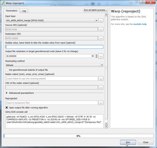
- In the search engine of the Processing Toolbox, type warp and select Warp (reproject) under Projections of GDAL.
- Under the Parameter tab, select the dem file as input layer.
- Select EPSG:4326 (WGS84 / Long Lat) under the Source SRS tab.
- Select EPSG:32632 (WGS84 /UTM Zone 32 N) under the Target SRS tab.
- Enter 30 as the output file resolution in meters.
- Select the Resampling method bilinear.
- Specify the Path and name of the output file.
- Click on Run to execute the algorithm.
[edit] Clipping of DEM data
- Create a boundary polygon
- Add the raster map geodata/raster/s2/Subset_S2A_MSIL2A_20170619T_MUL.tif
- In the search engine of the Processing Toolbox, type envelope and select Image Envelope under Geometry of OTB.
- Under the Parameter tab, select the raster file as input layer.
- In the Projection text field type 32632 (WGS84 /UTM Zone 32 N).
- Specify the Path and name of the output file.
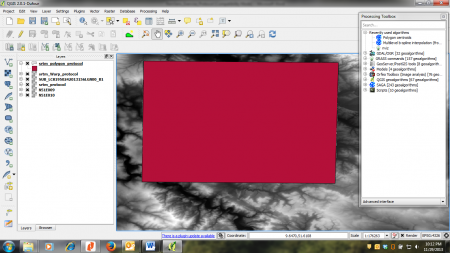
- Click on Run to execute the algorithm the layer is added to the canvas (figure C).
- Buffer the boundary polygon
- Choose Vector --> Geoprocessing tools --> Fixed distance buffer.
- Select the boundary polygon created before as input.
- Type 300 as buffer Distance in meters.
- Select name and output directory under Output shapefile.
- Confirm with OK and let the output layer be added to the canvas. Place it below the boundary polygon in the TOC to see the effect of buffering.
- Clipping the DEM map
- Open the clipping tool under Raster --> Extraction --> Clipper. Select the reprojected DEM file as input and select the output directory and file name as usual. Select the Mask layer radio button to select the buffered boundary layer as blueprint for clipping.
- Don't forget to check Crop the extent of the target dataset to the extent of the cropline.
- Enter an output path and file name. Confirm with OK.
- Map visualization
- Open the raster layer properties by right-clicking the clipped DEM map in the TOC and selecting Properties, or by simply double clicking.
- Select the Style tab. Under Render type select Singleband pseudocolor.
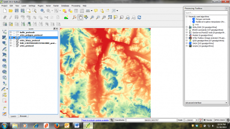
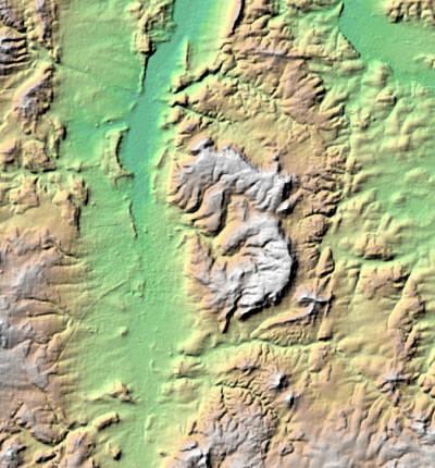
- In the Generate new color map section select Spectral. In the Mode pulldown menu select Equal interval. Set the number of Classes to 20 and click Classify.
- To finish, click Apply. If your're content with you settings, click OK to close the window (figure D).
[edit] Shaded relief layer styling
- Add a digital terrain model layer.
- Right click on the layer name and then click Duplicate from the menu
- Open the layer settings menu. Go to Style and change the render type to Hillshade and press OK
- Right click on the duplicated file Copy and open the layer settings menu.
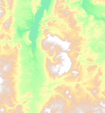
- Change the render type to Singleband Pseudocolor and select new color ramp. Select the color ramp type cpt-city. OK.
You'll find many more selections of color ramps sorted by theme. Select one (e.g. Topography > elevation). OK.
- Change Blending mode under Color rendering to Burn.
- Change layer transparency to 30%.
[edit] Computing hillshade, slope and aspect
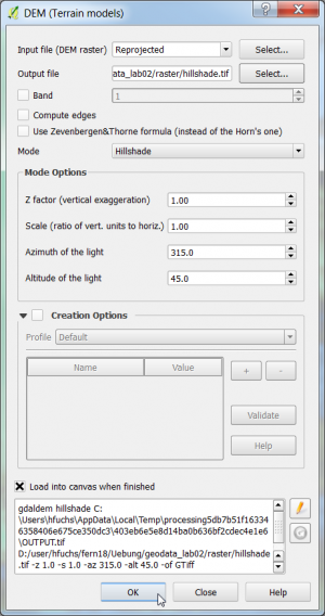
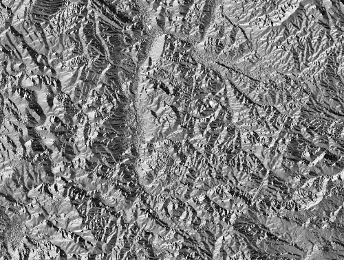
- Raster --> Analysis --> DEM (Terrain...)
- Add the reprojected DEM (WGS84 /UTM Zone 32 N).
- Select this dem file as input layer.
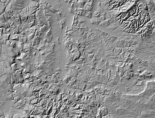
- Specify an output file hillshade.tif.
- Choose the mode Hillshade. OK.
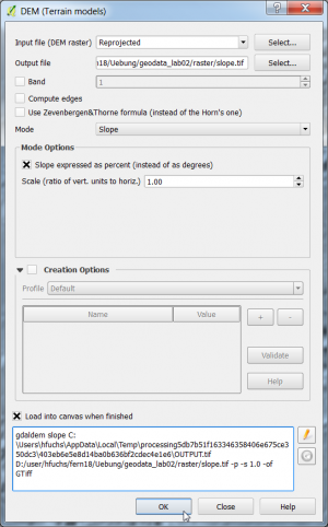
- Switch mode to Slope.
- Check Slope expressed as percent.
- Specify a new output file slope.tif. OK.
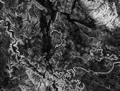
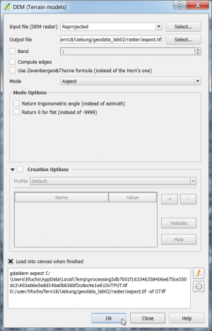
- Switch mode to Aspect.
- Specify a new output file aspect.tif. OK.
[edit] Trafficability slope classes
The following classification scheme for slope is given:
       Code    Slope[%]
       1        0- 5
       2        5-20
       3       20-30
       4       30-45
       5         >45
- Add slope as raster layer
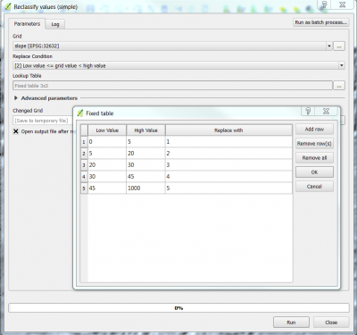
- In the search engine of the Processing Toolbox, type reclassify and select Reclassify values (simple) under Raster Tools of SAGA.
- Under the Parameter tab, select the slope layer as Grid.
- Select [2] Low value <= grid value < high value under the Replace condition tab.
- Enter the fixed table as shown below.
- Specify path and name of the output file.
- Click on Run to execute the algorithm.
- Render the changed grid with type Singleband Pseudocolor color ramp.
