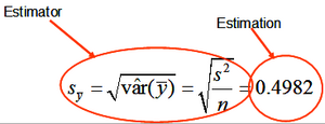
Statistical estimations
| (5 intermediate revisions by 2 users not shown) | |||
| Line 38: | Line 38: | ||
The “ ^ ” is generally used to make clear that an expression is a sample based estimation. If, for example the variance of variable <math>X</math> is denoted <math>var(X)</math>, then the estimated variance of <math>X</math> would be written as <math>\hat{var}(X)</math>. For the estimated mean and the estimated variance, one could also write <math>\hat\mu</math> and <math>\hat\sigma^2</math>, respectively. | The “ ^ ” is generally used to make clear that an expression is a sample based estimation. If, for example the variance of variable <math>X</math> is denoted <math>var(X)</math>, then the estimated variance of <math>X</math> would be written as <math>\hat{var}(X)</math>. For the estimated mean and the estimated variance, one could also write <math>\hat\mu</math> and <math>\hat\sigma^2</math>, respectively. | ||
| − | There are various important desirable characteristics of ''estimators'', among them unbiasedness and relative efficiency (when comparing to other estimators) | + | There are various important desirable characteristics of ''estimators'', among them [[Bias|unbiasedness]] and [[relative efficiency]] (when comparing to other estimators). It is emphasized here that these are properties of the estimators, not of the estimations! |
| − | + | ||
| − | + | ||
| − | + | ||
| − | + | ||
| − | + | ||
| − | + | ||
| − | + | ||
| − | + | ||
| − | + | ||
| − | + | ||
==Point estimates vs. interval estimates== | ==Point estimates vs. interval estimates== | ||
| − | For each statistic that is been estimated (such as a mean, a variance, a correlation coefficient, …) there are two basic types of statistical estimations, the “point estimate”, which estimates the parameter of interest, and the “interval estimate” which estimates the precision of the point estimate. The [[standard error]] is a measure of the variability of estimation | + | For each statistic that is been estimated (such as a mean, a variance, a correlation coefficient, …) there are two basic types of statistical estimations, the “point estimate”, which estimates the parameter of interest, and the “interval estimate” which estimates the precision of the point estimate. The [[standard error]] is a measure of the variability of estimation and defines the [[confidence interval]] of an estimate. |
| − | + | ||
| − | + | ||
| − | + | ||
| − | + | ||
| − | + | ||
| − | + | ||
| − | + | ||
| − | + | ||
| − | + | ||
| − | + | ||
| − | + | ||
==References== | ==References== | ||
Latest revision as of 09:59, 28 October 2013

We are interested to know the true population parameters but are not able to determine them. We use, therefore, sampling to produce estimations which we take then as approximations for the true population values; always knowing that estimations carry an error.
Estimations are the principal result of sampling studies. All results of a sample are estimations and must be interpreted as such; they help us to learn something about the unknown parameters of the population of interest.
[edit] Notations
There are some conventions in what refers to the notation of population parameters and estimated statistics:
| parametric mean | \(\mu\,\) |
| estimated mean | \(\bar{y}\,\) |
| parametric variance | \(\sigma^2\,\) |
| estimated variance | \(s^2\,\) |
| regression coefficients | \(\beta\,\) |
| estimated coefficients | \(b\,\) |
| unknown population parameter | \(\theta\,\) |
| sample based estimation | \(\hat\theta\,\) |
The “ ^ ” is generally used to make clear that an expression is a sample based estimation. If, for example the variance of variable \(X\) is denoted \(var(X)\), then the estimated variance of \(X\) would be written as \(\hat{var}(X)\). For the estimated mean and the estimated variance, one could also write \(\hat\mu\) and \(\hat\sigma^2\), respectively.
There are various important desirable characteristics of estimators, among them unbiasedness and relative efficiency (when comparing to other estimators). It is emphasized here that these are properties of the estimators, not of the estimations!
[edit] Point estimates vs. interval estimates
For each statistic that is been estimated (such as a mean, a variance, a correlation coefficient, …) there are two basic types of statistical estimations, the “point estimate”, which estimates the parameter of interest, and the “interval estimate” which estimates the precision of the point estimate. The standard error is a measure of the variability of estimation and defines the confidence interval of an estimate.
[edit] References
- ↑ Kleinn, C. 2007. Lecture Notes for the Teaching Module Forest Inventory. Department of Forest Inventory and Remote Sensing. Faculty of Forest Science and Forest Ecology, Georg-August-Universität Göttingen. 164 S.