Digital Elevation Model (DEM) Processing

Revision as of 12:29, 16 September 2014

In this article you will learn how to pre-process and enhance digital elevation model (DEM) data, as well as how to create a 3D-Model

Loading, merging and reprojection of DEM data

1. Add the raster layers N51E009.hgt and N51E010.hgt to a new QGIS project (from geodata\raster\DEM, see Course data). Arrange the first above the latter layer.
2. Merging layers
   • Select Raster --> Miscellaneous --> Merge. In the appearing menu, click the Select beside the Input files field. Browse for the maps N51E009.hgt and N51E010.hgt and select both (by clicking with pressed Ctrl key) (figure A).
   • Select an output directory and file name (e.g. N510_merged) under Output file. Confirm with OK.
3. Reprojecting layers (warp)
   • Select Raster --> Projections --> Warp (reprojects).
   • As Input file choose the merged layer from the preceding step. Select an according path and file name for Output file.
   • Determine the correct source and target spatial reference system (Source SRS and Target SRS) -- The coordinate system of the source layer is WGS84 (EPSG:4326). Use UTM32 (EPSG:32632) as target (figure B).
   • Confirm with OK.

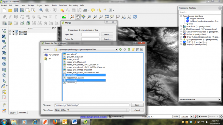Figure A: Merge dialogue and file browser in QGIS 2.0

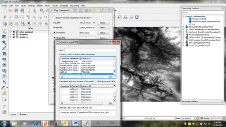Figure B: Warp dialogue and menu for SRS selection in QGIS 2.0

Clipping and Resampling of DEM data

1. Create a boundary polygon
   1. Add the raster map geodata/raster/landsat/landsat8/DOY156/SUB_LC81950242013156LGN00_B1 from the course data to the project.
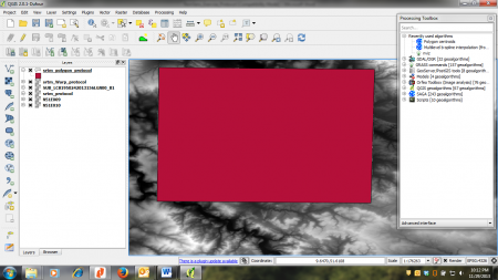
   2. Select Vector --> Research tools --> Polygon from layer extent. Choose the landsat map as input, select an output path and file name and confirm with OK. Confirm the following prompt to let the layer be added to the canvas (figure C).
2. Buffer the boundary polygon
   • Choose Vector --> Geoprocessing tools --> Buffer and select the boundary polygon created before as input. Select a reasonable name and output directory under Output shapefile. Confirm with OK and let the output layer be added to the canvas. Place it below the boundary polygon in the TOC to see the effect of buffering.
3. Clip the DEM map
   • Open the clipping tool under Raster --> Extractions --> Clipper. Select the reprojected DEM file as input and select the output directory and file name as usual. Select the Mask layer radio button to select the buffered boundary layer as blueprint for clipping. Don't forget to enter an output path and file name. Confirm with OK and let the result be added to the map.
4. Map visualization
   1. Open the raster layer properties by right-clicking the clipped DEM map in the TOC and selecting Properties, or by simply double clicking.
   2. Select the Style tab. Under Render type select Singleband pseudocolor.
   3. In the Generate new color map section select Spectral. In the Mode pulldown menu select Continuous. Set the number of Classes to 10 and click Classify.
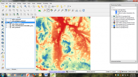
   4. To finish, click Apply. If your're content with you settings, click OK to close the window (figure D).
5. SAGA tools for resampling
   1. If not open, activate the processing toolbox by selecting Processing --> Toolbox.
   2. In the toolbox, browse for SAGA --> Grid-Spline --> Multilevel B-Spline Interpolation (from grid) or simply type Multilevel into the search field to find the tool. Open it with a double-click.
   3. In the appearing menu, select the following options:
      • The clipped layer from the Grid pulldown menu.
      • For the Output extent, select the clipped layer by clicking ... and selecting Use layer/canvas extent.
      • Set the Cell size to 30.
      • In the Grid input field at the bottom of the menu, select the directory and name for the output file.
      • Choose an output name and directory.
      • Leave the rest of the menu points as they are and click Run. The resampled layer will be added to the canvas.

Figure C: Boundary polygon produced by polygon to layer

Figure D: Clipped DEM map displayed in pseudocolor

3D visualization fo DEM data

1. Select GRASS --> Visualization --> nviz from the processing toolbox.
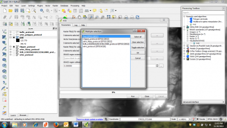
2. As Raster file(s) for elevation select the resampled DEM gridfile and confirm with OK (figure E).
3. Set the GRASS region cellsize to 1000.
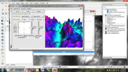
4. Click Run to start the algorithm. A new window will appear with a 3D-view of the DEM grid (figure F). The angles can be adjusted to change the perspective.

Figure E: NVIZ plugin menu

Figure F: 3D view of a DEM computed by the NVIZ plugin