File list
This special page shows all uploaded files. When filtered by user, only files where that user uploaded the most recent version of the file are shown.
| Name | Thumbnail | Size | User | Description | Versions | |
|---|---|---|---|---|---|---|
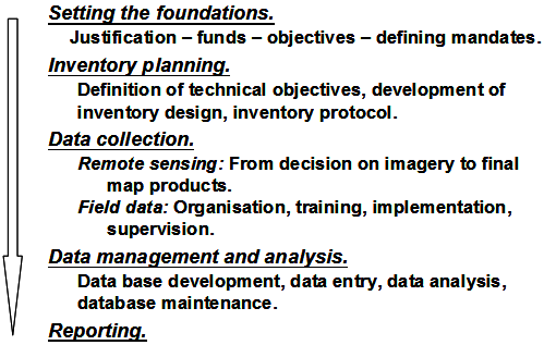
| 19:30, 18 March 2011 | 8.1.3-fig113.png (file) |  | 465 KB | Aspange | (General procedure of forest inventory planning. Reference: Kleinn, C. 2007. Lecture Notes for the Teaching Module Forest Inventory. Department of Forest Inventory and Remote Sensing. Faculty of Forest Science and Forest Ecology, Georg-August-Universitä) | 1 |
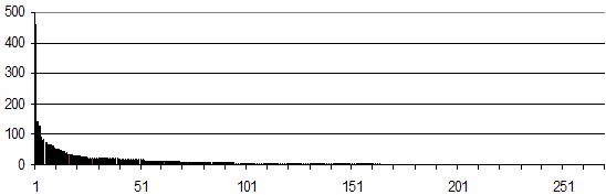
| 18:09, 18 March 2011 | 6.4.1-fig112.png (file) |  | 285 KB | Aspange | (Typical example for the distribution of species in a natural forest where the about 270 observed species were ordered by the number of observed individuals: some few species occur in larger numbers but there are also many species that are only observed on) | 1 |
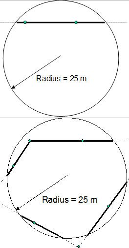
| 23:19, 16 March 2011 | 6.3.3-fig111.png (file) |  | 391 KB | Aspange | (Example for mapping forest boundary on circular plots: forest edges are surveyed on 25m radius plots that intersect with the forest boundary. One plot is assumed to contain a maximum of two border lines that are to be measured. If the forest boundary is a) | 1 |
| 22:20, 16 March 2011 | 6.2.3-fig110.png (file) |  | 246 KB | Aspange | (Line sampling with different sampling elements: straight line, L-shape and square in an area that consists to 50% of forest. Total line length is fixed in the left figure and adjusted to the buffer strip (that is: the maximum extension of the line is equa) | 1 |
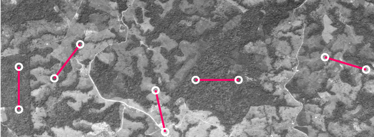
| 22:19, 16 March 2011 | 6.2.3-fig109.png (file) |  | 586 KB | Aspange | (Two approaches of area estimation when line sampling is used: #either the entire line is used for line intercept sampling, or #only the end points are observed, so that the observation unit is actually a cluster of two points at a defined distance away ) | 1 |
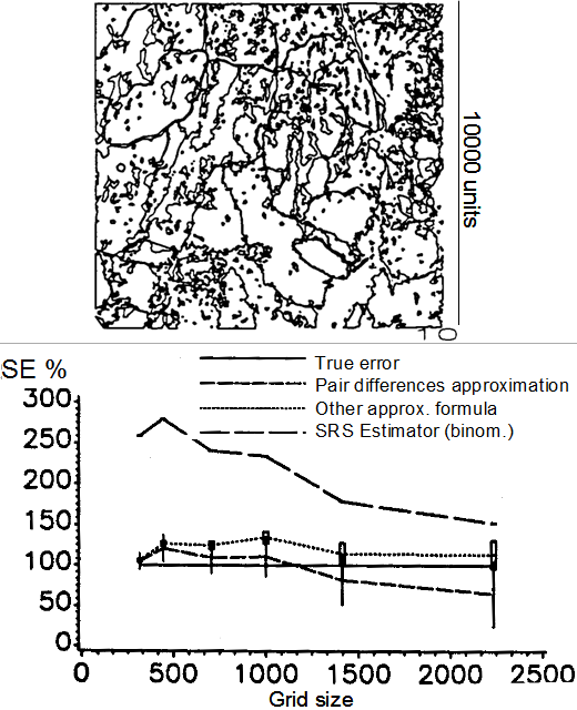
| 22:05, 16 March 2011 | 6.2.2-fig108.png (file) |  | 977 KB | Aspange | (Comparison of empirically derived standard error with other approximation methods. Above: sample map. Below: results. References: Kleinn C. 1991. Der Fehler von Flächenschätzungen mit Punkterastern und linienförmigen Stichprobenelementen. Disserta) | 1 |
| 20:28, 16 March 2011 | 6.1.4-fig107.png (file) |  | 242 KB | Aspange | (Plot combination schemes in sampling with partial replacement. Reference: Kleinn, C. 2007. Lecture Notes for the Teaching Module Forest Inventory. Department of Forest Inventory and Remote Sensing. Faculty of Forest Science and Forest Ecology, Georg-Aug) | 1 |
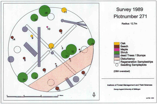
| 12:52, 11 March 2011 | 6.1.2-fig106.png (file) |  | 498 KB | Aspange | (Example of a mapped plot. Reference: Brändli U.B., A. Herold, H. Stierlin und J. Zinggeler 1994. Schweizerisches Landesforst-inventar. Anleitung für die Feldaufnahmen der Erhebung 1993-1995. Birmensdorf, Eidg. Forschungsanstalt für Wald, Schnee und L) | 1 |
| 12:51, 11 March 2011 | 6.1.2-fig105.png (file) |  | 408 KB | Aspange | (Permanent plot where trees measured twice are depicted. Reference: Brändli U.B., A. Herold, H. Stierlin und J. Zinggeler 1994. Schweizerisches Landesforst-inventar. Anleitung für die Feldaufnahmen der Erhebung 1993-1995. Birmensdorf, Eidg. Forschungsa) | 1 |
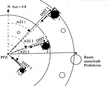
| 12:44, 11 March 2011 | 6.1.2-fig104.png (file) |  | 436 KB | Aspange | (Referencing and recording of individual tree in a permanent plot. Reference: Brändli U.B., A. Herold, H. Stierlin und J. Zinggeler 1994. Schweizerisches Landesforst-inventar. Anleitung für die Feldaufnahmen der Erhebung 1993-1995. Birmensdorf, Eidg. F) | 1 |
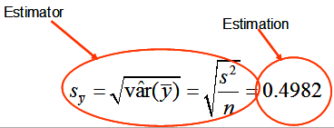
| 23:41, 9 March 2011 | 3.5-fig00.png (file) |  | 152 KB | Aspange | (The estimator is the calculation algorithm (formula) that produces the estimation. Reference: Kleinn, C. 2007. Lecture Notes for the Teaching Module Forest Inventory. Department of Forest Inventory and Remote Sensing. Faculty of Forest Science and Fores) | 1 |
| 23:27, 9 March 2011 | 3.7-fig44.png (file) |  | 767 KB | Aspange | (Distribution of sample based estimations of deforestation for Bolivia with 10% sampling intensity. Left: a wide range of estimated deforestation figures is produced when the original 41 Landsat scenes are taken as population. However, when these 41 images) | 1 |
| 22:44, 9 March 2011 | 4.1.1-fig45.png (file) |  | 398 KB | Aspange | (Typical shape of a spatial autocorrelation function. Here, however, the covariance is given. The correlation would look exactly the same, but with a y-axis re-scaled to the range of 0.0 to 1.0. Reference: Kleinn, C. 2007. Lecture Notes for the Teaching ) | 1 |
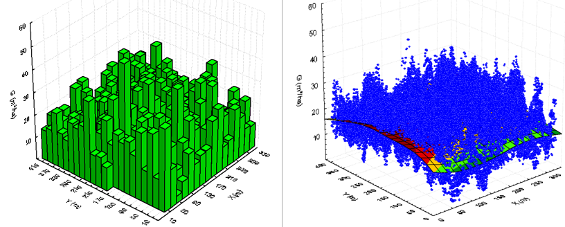
| 21:45, 9 March 2011 | 4.8-fig70.png (file) |  | 786 KB | Aspange | (Illustration of approaches for plot populations for the same example population. Left: discrete population of square sample plots with defined positions. Right: each point in the area is a sampling element the value of which is determined by the surroundi) | 1 |
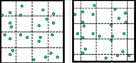
| 21:32, 9 March 2011 | 4.8-fig69.png (file) |  | 302 KB | Aspange | (An identical “forest area” subdivided in two different ways in square sample plots of the same basic size. Right: plot fragments occur along the border line. The total of “number of stems” is obviously identical in both cases; but this is not the ) | 1 |
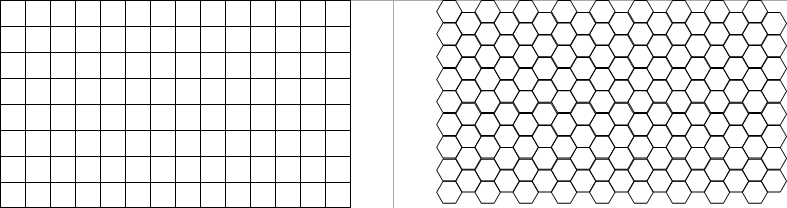
| 21:27, 9 March 2011 | 4.8-fig68.png (file) | 481 KB | Aspange | (Illustration of approach 1 for plot populations: subdivision of the forest area into sample plots of identical shape and size, here: square and hexagonal sample plots. Such a subdivision is also possible for rectangles and some types of triangles. Refere) | 1 | |
| 23:19, 7 March 2011 | 4.5.3-fig66.png (file) |  | 372 KB | Aspange | 1 | |
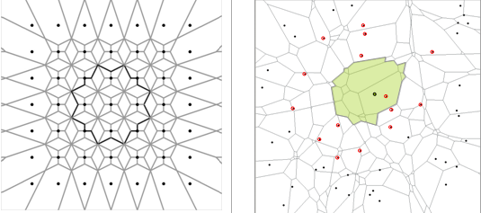
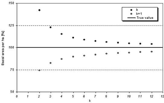
| 22:55, 7 March 2011 | 4.5.1-fig65.png (file) |  | 545 KB | Aspange | (Illustration why the simple expansion factor approach does produce a systematic overestimation for ''k''-tree sampling. Reference: Kleinn, C. 2007. Lecture Notes for the Teaching Module Forest Inventory. Department of Forest Inventory and Remote Sensing) | 1 |
| 22:48, 7 March 2011 | 4.5.1-fig64.png (file) |  | 281 KB | Aspange | (Illustration why the simple expansion factor approach does produce a systematic overestimation for k-tree sampling. Reference: Kleinn, C. 2007. Lecture Notes for the Teaching Module Forest Inventory. Department of Forest Inventory and Remote Sensing. Fa) | 1 |
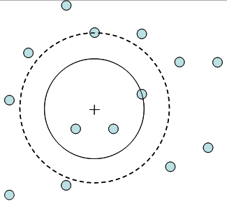
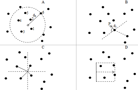
| 22:46, 7 March 2011 | 4.5.1-fig63.png (file) |  | 399 KB | Aspange | (Some variations of ''k''-tree sampling. Reference: Kleinn, C. 2007. Lecture Notes for the Teaching Module Forest Inventory. Department of Forest Inventory and Remote Sensing. Faculty of Forest Science and Forest Ecology, Georg-August-Universität Götti) | 1 |
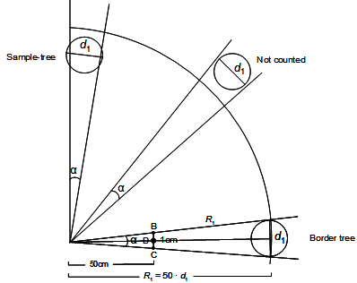
| 21:32, 5 March 2011 | 4.4.2-fig62.png (file) |  | 254 KB | Aspange | (Critical angle principle. Reference: Kleinn, C. 2007. Lecture Notes for the Teaching Module Forest Inventory. Department of Forest Inventory and Remote Sensing. Faculty of Forest Science and Forest Ecology, Georg-August-Universität Göttingen. 164 S.) | 1 |
| 20:46, 5 March 2011 | 4.3-fig58.png (file) |  | 681 KB | Aspange | 2 | |
| 20:44, 5 March 2011 | 4.4.2-fig60.png (file) |  | 369 KB | Aspange | 2 | |
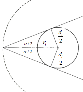
| 20:42, 5 March 2011 | 4.4.2-fig61.png (file) |  | 228 KB | Aspange | (Illustration of calculation of the radius of the virtual circular sub-plot for a tree with diameter <math>d_i</math>. Reference: Kleinn, C. 2007. Lecture Notes for the Teaching Module Forest Inventory. Department of Forest Inventory and Remote Sensing. ) | 1 |
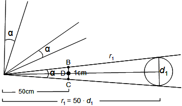
| 20:32, 5 March 2011 | 4.4.1-fig59.png (file) |  | 273 KB | Aspange | (Illustration of selection proportional to size (basal area) in Bitterlich sampling. Reference: Kleinn, C. 2007. Lecture Notes for the Teaching Module Forest Inventory. Department of Forest Inventory and Remote Sensing. Faculty of Forest Science and Fore) | 1 |
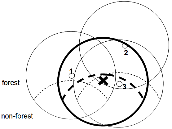
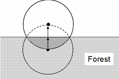
| 20:14, 5 March 2011 | 4.3-fig57.png (file) |  | 492 KB | Aspange | (Principle of the mirage method for border plot correction. The center of the plot is mirrored at the forest edge outside the forest. From that new point, again a circular plot is laid out and all trees tallied again which fall into it; these trees are obs) | 2 |
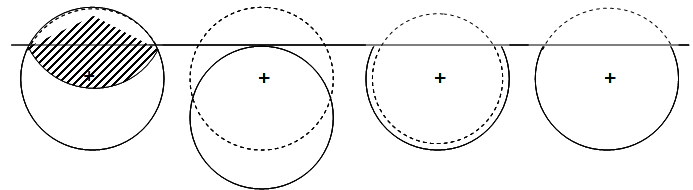
| 20:11, 5 March 2011 | 4.3-fig56.png (file) | 387 KB | Aspange | (Different techniques applied to boundary plots. Only the mirage technique is not causing a systematic error. From left to right: mirage method, shifting the plot, enlarging the circular plot at the same location such that the plot area is maintained, and ) | 1 | |
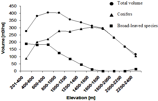
| 09:16, 3 March 2011 | 4.2.6.2-fig55.png (file) |  | 531 KB | Aspange | (Volume over elevation estimated from the second Swiss National Forest Inventory. Reference: Kleinn C., B. Traub and C. Hoffmann 2002. A note on the slope correction and the estimation of the length of line features. Canadian Journal of Forest Research 3) | 1 |
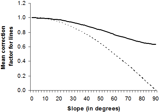
| 09:02, 3 March 2011 | 4.2.6.1-fig54.png (file) |  | 539 KB | Aspange | (Mean correction factor for line features as a function of terrain inclination a (bold line), assuming that the lines have a uniform distribution of angular deviation from the gradient vector. The dashed line gives the standard correction factor cos(<math>) | 1 |
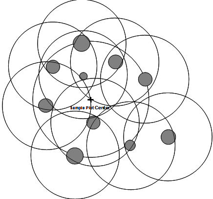
| 08:35, 3 March 2011 | 4.2.2-fig47.png (file) |  | 520 KB | Aspange | (Illustration of the inclusion zone approach: For fixed area circular plots, the inclusion zones are identical for all trees. Those trees are taken as sample trees in whose inclusion zones the sample point comes to lie. Reference: Kleinn, C. 2007. Lectur) | 2 |
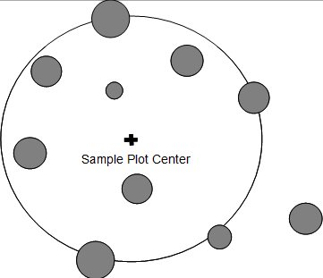
| 08:34, 3 March 2011 | 4.2.2-fig46.png (file) |  | 330 KB | Aspange | (With circular sample plots all trees are taken as sample trees that are within a defined distance (radius) from the sample point, which constitutes the plot center. Reference: Kleinn, C. 2007. Lecture Notes for the Teaching Module Forest Inventory. Depa) | 2 |
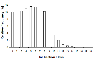
| 08:30, 3 March 2011 | 4.2.6-fig53.png (file) |  | 272 KB | Aspange | (Distribution of inclination of forest plots of the second Swiss National Forest Inventory (class 0, 0-9.99%, class 1, 10-19.99%, etc.) Reference: Kleinn C., B. Traub and C. Hoffmann 2002. A note on the slope correction and the estimation of the length ) | 1 |
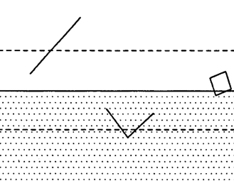
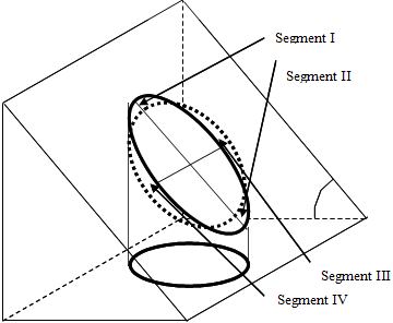
| 08:10, 3 March 2011 | 4.2.6-fig52.png (file) |  | 313 KB | Aspange | (A diagram showing an area of refer-ence and projected area into the map plane on a sloping terrain. Reference: Kleinn C., B. Traub and C. Hoffmann 2002. A note on the slope correction and the estimation of the length of line features. Canadian Journal o) | 1 |
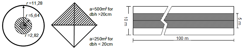
| 07:57, 3 March 2011 | 4.2.2-fig51.png (file) | 398 KB | Aspange | (Different combination of shapes for nested sub-plots. Reference: Prodan M., R. Peters, F. Cox and P. Real 1997. Mensura forestal. Serie investigación y educación en desarrollo sostenible. IICA/GTZ. 561p.) | 1 | |
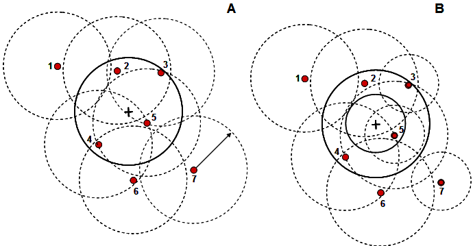
| 07:53, 3 March 2011 | 4.2.2-fig50.png (file) |  | 727 KB | Aspange | (Comparison of the inclu-sion zone approach for nested circular sub-plots (B) and for fixed circu-lar plots (A). Reference: Kleinn, C. 2007. Lecture Notes for the Teaching Module Forest Inventory. Department of Forest Inventory and Remote Sensing. Facult) | 1 |
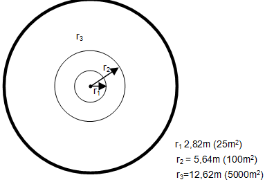
| 07:52, 3 March 2011 | 4.2.2-fig49.png (file) |  | 296 KB | Aspange | (Nested sub-plots showing 3 circular plots having different sizes, radii, but sharing same plot center Reference: Kleinn, C. 2007. Lecture Notes for the Teaching Module Forest Inventory. Department of Forest Inventory and Remote Sensing. Faculty of Fores) | 1 |
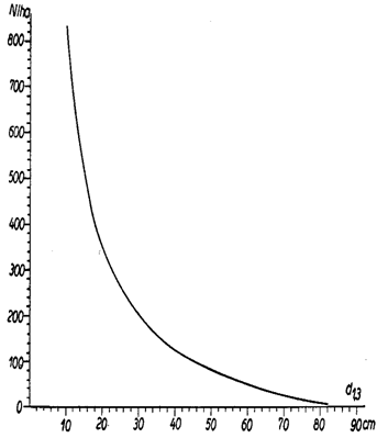
| 07:51, 3 March 2011 | 4.2.2-fig48.png (file) |  | 402 KB | Aspange | (Typical diameter distribution in a natural forest. Reference: Kleinn, C. 2007. Lecture Notes for the Teaching Module Forest Inventory. Department of Forest Inventory and Remote Sensing. Faculty of Forest Science and Forest Ecology, Georg-August-Universi) | 1 |
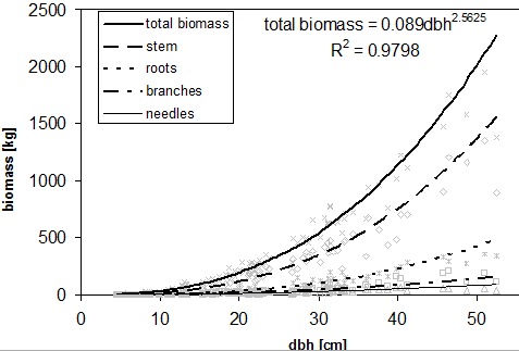
| 23:45, 1 March 2011 | 2.8.5-fig43.png (file) |  | 452 KB | Aspange | (Allometric functions for different tree compartments and total biomass for a Norway spruce dataset. Reference: Kleinn, C. 2007. Lecture Notes for the Teaching Module Forest Inventory. Department of Forest Inventory and Remote Sensing. Faculty of Forest ) | 1 |
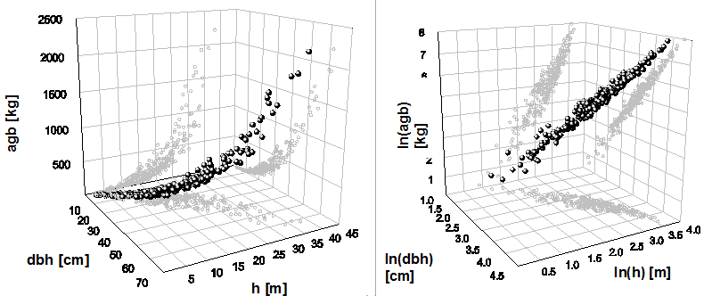
| 23:43, 1 March 2011 | 2.8.5-fig42.png (file) |  | 770 KB | Aspange | (Relationship between dbh, tree height and aboveground biomass on a metric (original) scale (left) and after logarithmic transformation of the variables (right) Reference: Kleinn, C. 2007. Lecture Notes for the Teaching Module Forest Inventory. Departmen) | 1 |
| 21:58, 1 March 2011 | 2.8.4-fig40.png (file) |  | 1.31 MB | Aspange | (Schematic graphs of confidence intervals for the case of equal variances (left) and the unequal variances case as it presents itself with volume functions (right). Reference: Kleinn, C. 2007. Lecture Notes for the Teaching Module Forest Inventory. Depar) | 1 |
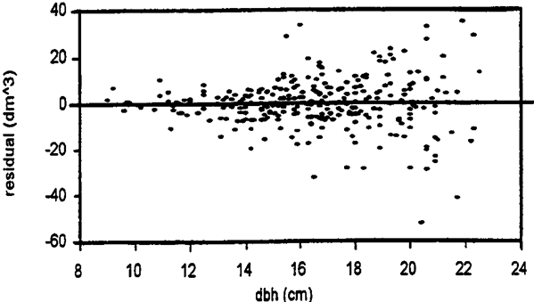
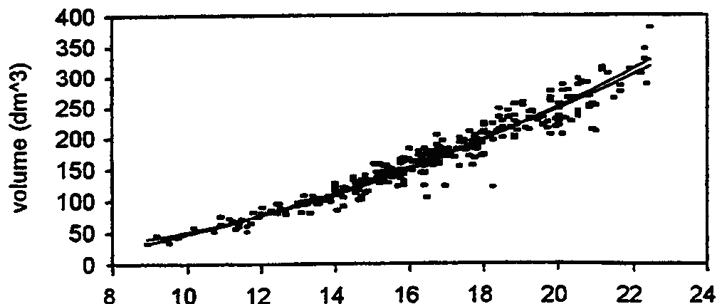
| 21:46, 1 March 2011 | 2.8.4-fig39.png (file) |  | 596 KB | Aspange | (Residual plot of residual volume (<math>dm^3</math> as Y-axis and ''dbh'' (cm) as X-axis showing unequal variance across ''dbh'' classes Reference: Kleinn, C. 2007. Lecture Notes for the Teaching Module Forest Inventory. Department of Forest Inventory ) | 1 |
| 20:53, 18 February 2011 | 2.8.4-fig38.png (file) |  | 425 KB | Aspange | 1 | |
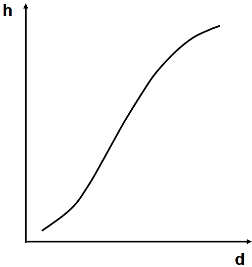
| 20:23, 18 February 2011 | 2.8.3-fig37.png (file) |  | 774 KB | Aspange | (A typical height curve in a natural uneven-aged stand. If the forest is in a “steady state”, This curve does not change over time and can simultaneously be interpreted as growth curve. Reference: Prodan M., R. Peters, F. Cox and P. Real. 1997.Mensur) | 1 |
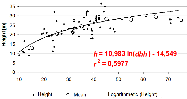
| 19:14, 18 February 2011 | 2.8.3-fig36.png (file) |  | 480 KB | Aspange | (The same height curve as in Figure 2 but drawn in a grid with ln(''dbh'') on the abscissa instead of ''dbh'' only.) | 1 |
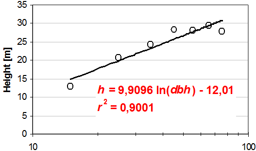
| 19:08, 18 February 2011 | 2.8.3-fig35.png (file) |  | 825 KB | Aspange | (Simple linear regression with ln(dbh) as sole independent variable. In addition to the data points, the mean heights per 10cm dbh-class are given. In this case, the model is obviously not flexible enough to adjust well to the height values for very large ) | 1 |
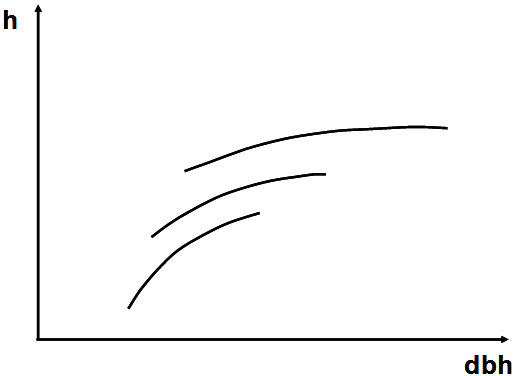
| 19:07, 18 February 2011 | 2.8.3-fig34.png (file) |  | 568 KB | Aspange | (Height curves in even aged stands exhibit typical changes over time which are depicted here simplified and schematically: they get flatter, shift right on the dbh axis and up on the height axis and cover a wider range of diameters (“become longer”).) | 1 |
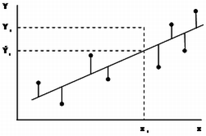
| 18:41, 18 February 2011 | 2.8.2-fig33.png (file) |  | 175 KB | Aspange | (Illustration of the least squares technique. The distance which is squared is not the perpendicular one but the distance in <math>y</math>-direction as we are interested in predictions over given values of <math>x</math>.) | 2 |
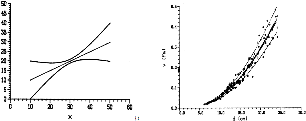
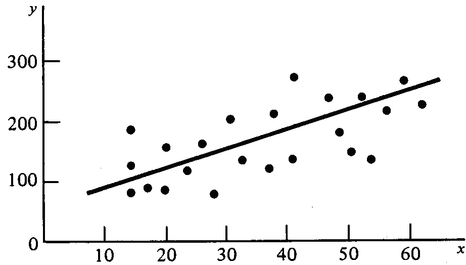
| 18:26, 18 February 2011 | 2.8.2-fig32.png (file) |  | 474 KB | Aspange | (Straight line representing a linear regression model between variable ''X'' and ''Y''.) | 1 |
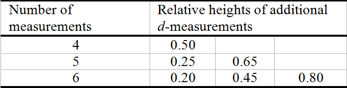
| 17:52, 18 February 2011 | 2.7.2.3-tab4.png (file) | 373 KB | Aspange | („Optimal“ distribution of measurement points along a stem to determine stem volume with highest precision by interpolation with cubic splines. Three measurement points are “fixed”: at 0.2 m height (assumed felling height), at 1.3 m (dbh) and total) | 1 | |
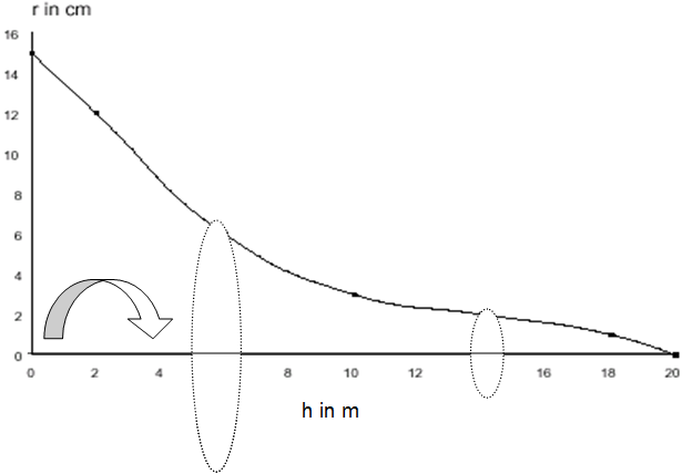
| 17:36, 18 February 2011 | 2.7.2.3-fig31.png (file) |  | 773 KB | Aspange | (Illustration of a taper curve which models the stem shape from the tree bottom (left) to the top (right). The radius is given as a function of tree height/stem length. By rotating this curve, we obtain a solid which is a model for the stem from which the ) | 1 |
First page |
Previous page |
Next page |
Last page |