File:Iterative Clustering.png
From AWF-Wiki

Size of this preview: 800 × 267 pixels.
Full resolution (2,400 × 800 pixels, file size: 113 KB, MIME type: image/png)
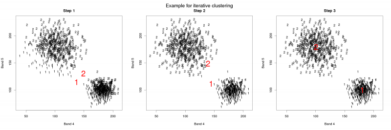
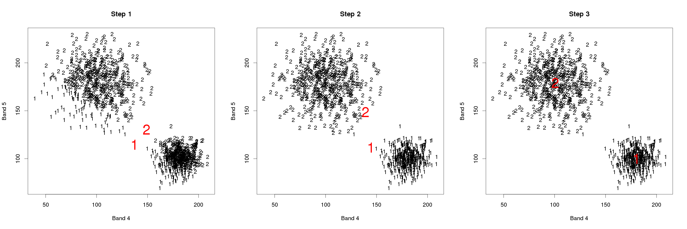
An example R plot to show the basic principle of iterative (migrating means) clustering. Code:
### Let us simulate iterative clustering!
## Note that the result can better be
# achieved by simply using the kmeans function:
# 	clust <- kmeans(data, 2)
# The following code only serves to create a
# single-step example.

## Some fictional satellite brightness values:
set.seed(23) # just change the seed to see different outcomes!

data <- data.frame(band.4=c(rnorm(500, mean=100, sd=20),
			    rnorm(500, mean=180, sd=10)),
		   band.5=c(rnorm(500, mean=180, sd=20),
			    rnorm(500, mean=100, sd=10)))


## make a fictional cluster
# first we need two random means (for two classes)

clmeans <- data.frame(band.4=runif(2, min(data$band.4),
					  max(data$band.4)),
		      band.5=runif(2, min(data$band.5),
				   max(data$band.5)))

## function for calculating distances to means
cldist <- function(p, m){

	# attach means to point data frame
	dists.all <- as.matrix(dist(rbind(p, m)))

	# obtain distances of points to means
	l <- dim(dists.all)[1] # get width/length of matrix

	dists.m <- dists.all[(l-1):l, 1:(l-2)]


	return(data.frame(dists.1=dists.m[1,],
			  dists.2=dists.m[2,]))

}

# now apply function to data
data <- cbind(data, cldist(data, clmeans))

## assign points to class, depending on minimum distance
data$class <- ifelse(data$dists.1 < data$dists.2, 1, 2)

## same for means of new classes
clmeans.2 <- aggregate(list(band.4=data$band.4, band.5=data$band.5),
	  by=list(class=data$class), mean)[,2:3]

data.2 <- cbind(data[,1:2], cldist(data[,1:2], clmeans.2))

data.2$class <- ifelse(data.2$dists.1 < data.2$dists.2, 1, 2)

## one more step
clmeans.3 <- aggregate(list(band.4=data.2$band.4, band.5=data.2$band.5),
	  by=list(class=data.2$class), mean)[,2:3]

data.3 <- cbind(data.2[,1:2], cldist(data.2[,1:2], clmeans.3))

data.3$class <- ifelse(data.3$dists.1 < data.3$dists.2, 1, 2)


## plot
png('Iterative_Clustering.png', width=2400, height=800,
    pointsize=30)

op <- par(mfrow=c(1,3))
plot(data$band.4, data$band.5, type='n', xlab='Band 4', ylab='Band 5')
title('Step 1', line=1)
text(data$band.4, data$band.5, labels=as.character(data$class))
text(clmeans$band.4, clmeans$band.5, labels=c('1', '2'), col='red',
     cex=2.5)

plot(data.2$band.4, data.2$band.5, type='n', xlab='Band 4', ylab='Band 5')
text(data.2$band.4, data.2$band.5, labels=as.character(data.2$class))
text(clmeans.2$band.4, clmeans.2$band.5, labels=c('1', '2'), col='red',
     cex=2.5)
mtext("Example for iterative clustering", line=2)
title('Step 2', line=1)

plot(data.3$band.4, data.3$band.5, type='n', xlab='Band 4', ylab='Band 5')
text(data.3$band.4, data.3$band.5, labels=as.character(data.3$class))
text(clmeans.3$band.4, clmeans.3$band.5, labels=c('1', '2'),
     col='red', cex=2.5)
title('Step 3', line=1)

options(op)
dev.off()
File history
Click on a date/time to view the file as it appeared at that time.
| Date/Time | Thumbnail | Dimensions | User | Comment | |
|---|---|---|---|---|---|
| current | 12:05, 3 August 2013 | 2,400 × 800 (113 KB) | Lburgr (Talk | contribs) | Added main title. | |
| 11:32, 3 August 2013 | 2,400 × 800 (108 KB) | Lburgr (Talk | contribs) | An example R plot to show the basic principle of iterative (migrating means) clustering. Code: ### Let us simulate iterative clustering! ## Note that the result can better be # achieved by simply using the kmeans function: # clust <- kmeans(data,... |
- Edit this file using an external application (See the setup instructions for more information)
File usage
The following page links to this file: