|
|
| (13 intermediate revisions by one user not shown) |
| Line 21: |
Line 21: |
| | | 1 | | | 1 |
| | | Artificial surfaces | | | Artificial surfaces |
| − | | 1 | + | | 11 |
| | | Built-up | | | Built-up |
| | | 230-0-77 | | | 230-0-77 |
| Line 27: |
Line 27: |
| | | 2 | | | 2 |
| | | Agricultural | | | Agricultural |
| − | | 2 | + | | 22 |
| | | Arable land | | | Arable land |
| | | 255-255-168 | | | 255-255-168 |
| Line 33: |
Line 33: |
| | | 2 | | | 2 |
| | | Agricultural | | | Agricultural |
| − | | 3 | + | | 23 |
| | | Bare soil | | | Bare soil |
| | | 253-191-168 | | | 253-191-168 |
| Line 39: |
Line 39: |
| | | 2 | | | 2 |
| | | Agricultural | | | Agricultural |
| − | | 4 | + | | 24 |
| | | Pasture | | | Pasture |
| | | 230-230-77 | | | 230-230-77 |
| Line 45: |
Line 45: |
| | | 3 | | | 3 |
| | | Natural and semi-natural areas | | | Natural and semi-natural areas |
| − | | 5 | + | | 31 |
| | | Broad leaved tree cover | | | Broad leaved tree cover |
| | | 128-255-0 | | | 128-255-0 |
| Line 51: |
Line 51: |
| | | 3 | | | 3 |
| | | Natural and semi-natural areas | | | Natural and semi-natural areas |
| − | | 6 | + | | 32 |
| | | Coniferous tree cover | | | Coniferous tree cover |
| | | 0-166-0 | | | 0-166-0 |
| Line 57: |
Line 57: |
| | | 5 | | | 5 |
| | | Water | | | Water |
| − | | 7 | + | | 51 |
| | | Water | | | Water |
| | | 128-242-230 | | | 128-242-230 |
| | |- | | |- |
| − | | 0 | + | | 6 |
| | | Miscellaneous | | | Miscellaneous |
| − | | 8 | + | | 61 |
| − | | No data (cloud) | + | | Cloud |
| | | 255-255-255 | | | 255-255-255 |
| | |- | | |- |
| − | | 0 | + | | 6 |
| | | Miscellaneous | | | Miscellaneous |
| − | | 9 | + | | 62 |
| − | | No data (shadow) | + | | Cloud shadow |
| − | | 0-0-0 | + | | 100-50-0 |
| | |- | | |- |
| − | | 0 | + | | 6 |
| | | Miscellaneous | | | Miscellaneous |
| − | | 10 | + | | 63 |
| | | Unclassified | | | Unclassified |
| | | 0-0-0 | | | 0-0-0 |
| | |} | | |} |
| − |
| |
| − | ==Creating systematic sampling grid==
| |
| − | * A processing toolbox model can downloaded from Stud.IP {{typed|text=urban_atlas_systematic_sample.model3}} or by right click on [http://www.gwdg.de/~hfuchs/qgis/urban_atlas_systematic_sample.model3 here] and Save file as ...
| |
| − | * Open QGIS and go to the Processing Toolbox; if the Toolbox is not opened click {{mitem|text= Processing --> Toolbox}} to activate it.
| |
| − | * In the processing toolbar click {{button|text=Options}} [[File:qgis_processing_options.png]]. In the General tab choose "ignor invalid features with invalid geoemtries".
| |
| − | [[File:qgis_processing_invalid_feature.png|500px]]
| |
| − | * Go to [[File:qgis-processing_model_iconExample.png]] {{mitem|text= Models --> Open existing models}} and load the previously downloaded model. The model should appear in the Models tab. Double click on it to execute.
| |
| − | * Specify the ''European Urban Atlas Vector File'' layer for Göttingen: ''\lucc\DE021L1_GOTTINGEN\Subset-Goe_DE021L1_GOTTINGEN_UA2012_UTM32N.shp'' or download data from other [https://land.copernicus.eu/local/urban-atlas/urban-atlas-2012 European cities]. The original European Urban Atlas data have the spatial reference system EPSG:3035 (ETRS89, LAEA). The Goettingen Urban Atlas file is already transformed to WGS84 /UTM 32. There might occur geometry errors: Run {{mitem|text=Processing Toolbox --> Check validitiy}} and {{mitem|text=Processing Toolbox --> Fix geometries}} repairing invalid vector geometries.
| |
| − | * {{mitem|text=Project --> Project Properties --> CRS}}. Check that the Project spatial reference system is set to '''EPSG:32632'''.
| |
| − | [[File:qgis_goe_syst_sample.png|400px]]
| |
| − | * Click {{button|text=Run}}
| |
| − |
| |
| − | ==Stratified random sampling==
| |
| − | * {{mitem|text=Vector --> Research Tools --> Random selection within subsets}}
| |
| − | * The input layer is ''SCP_systematic_points''
| |
| − | * ID Field containing the code for the strata is '''MC_ID'''
| |
| − | * Method is equal ''Number of selected features'' in each stratum.
| |
| − | * Number of selected features type '''25'''.
| |
| − |
| |
| − | [[File:qgis_stratified_selection.png|400px]]
| |
| − |
| |
| − | The module selects a subset of the layer ''SCP_systematic_points''. The selected points need to be saved as an ESRI shapefile. Right click on the layer ''SCP_systematic_points'', {{button|text=Save as...}}. Make sure to check the box: '''Save selected only..''as shown below.
| |
| − |
| |
| − | [[File:qgis_save_selection.png|400px]]
| |
| − |
| |
| − | == Interpretation of selected points==
| |
| − |
| |
| − | Prepare main QGIS map viewer:
| |
| − | * Install the ''Openlayers'' and the ''Go2nextFeature3'' plugin (if not yet done) {{mitem|text=Plugins --> Manage and Install Plugins --> Install}}.
| |
| − | * Load the multiband Sentinel-2 satellite image ''Subset_S2A_MSIL2A_20170619T_MUL.tif''.
| |
| − | * Create a false-color composite (RGB = 9-7-3)(see [Changing Raster Layer Style]. Set the {{mitem|text=Layer Properies --> Transparency --> Global Transparency}} to 50%.
| |
| − | * Load the comma separated file with stratified sample points: ''CE_2020-01-03.csv''.
| |
| − | * Load Google maps as background WMS layer.
| |
| − | * In {{tool|text=Layers panel}} drag the Sentinel-2 image on top of ''Google Satellite''.
| |
| − | * Drag the sample points vector file on top of all other files.
| |
| − | * Activate {{mitem|text=Plugins -->Go 2 next feature}}.
| |
| − | * Layer is the sample points.
| |
| − | * The Attribute is ''Id''.
| |
| − | * Click the checkbox '''Select''' on.
| |
| − | [[File:qgis_go2nextfeature.png|400px]]
| |
| − | * In {{tool|text=Layers panel}} right click on the sample point layer and {{button|text=Open Attribute Table}}.
| |
| − | * On the lower left of the Attribute Table switch from {{button|text=Show All Features}} to {{button|text=Show Selected Features}}.
| |
| − | * Start the edit mode of the point layer by clicking the {{button|text=Toggle editing}} button [[file:QGIS_2.0_Edit.png|25px]].
| |
| − | * Arrange the windows on your Desktop as shown below.
| |
| − | [[File:qgis_goe_interpret_luc.png|1200px]]
| |
| − | * Enter the interpreted land cover class in column '''valid_cl''' of the Attribute Table.
| |
| − | * Do not forget to click {{button|text=Save edits}} button [[file:QGIS_2.0_SaveEdits.png|25px]].
| |
| − | * To stop the edit mode of the point layer click the {{button|text=Toggle editing}} button
| |
| − | * Export the file in format csv.
| |
| − | [[file:QGIS_2.0_Edit.png|25px]] again.
| |
| − |
| |
| − | [[category:QGIS Tutorial]]
| |
Before starting to map land cover classes using Sentinel-2 satellite images we need clear definitions and a classification scheme.
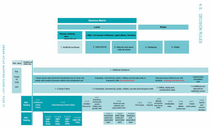
An example for a hierarchical land use and land cover (LUC) classification scheme is the European Urban Atlas.
The scheme defines 5 meta classes where the class 1. Artificial surfaces has many sub classes as shown in figure A.
The specification of other meta classes is not as detailed. If we are more interested in forest and open area classes we need to adapt and modify this scheme.
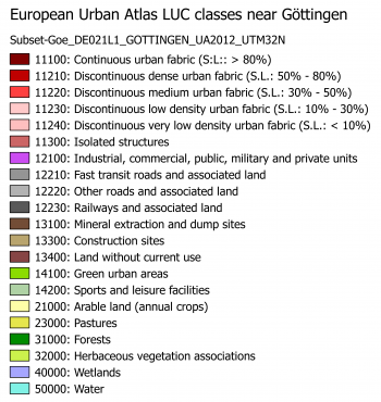
On the lowest level not all classes defined in the European Urban Atlas do also appear in the surroundings of Göttingen (figure B).
In addition we need to consider the phenolgical development of vegetation at specific acquisiton dates and to specify more classes which can possibly be identified in multispectral feature space of the satellite image.
An example of an adapted simplified scheme is shown in the table below.

