Systematic sampling
Contents |
General descriptions of systematic sampling
Systematic sampling is a name of a wide class of sampling strategies in which selection of individual elements is following a systematic pattern. Examples are square grids of sample points laid out over an area of interest; or the selection of every 10th tree in an alley; or parallel transects.
Systematic sampling and its applications to forest inventory are best illustrated with square grids of sample points. We may imagine a transparency sheet on which this grid is printed; and this transparency is placed randomly over the map, where randomly means: randomly selected starting point and random orientation. From a sample selection point of view, it is important to state that we have only one independent selection of a sample point; after having selected the first point, all others are fixed. We defined earlier that sample size is the number of independently selected elements; an immediate conclusion is that systematic sampling is obviously a sample of size \(n = 1\). The “plot” that is being laid out then is a large cluster plot consisting of numerous sub-plots – that is, all the sample points on the systematic sample are strictly spoken sub-plots of one single cluster that is spread out over the entire area.
A major question is then whether we can make an unbiased estimation of mean and variance from a random sample of size \(n = 1\). For the estimation of the mean, there is no problem at all: the estimator
\(\bar y=\frac{\sum_{i=1}^n y_i}{n}\,\)
can be calculated and yields the estimation of the mean.
However, when we wish to estimate the variance with the estimator
\(s^2=\frac{\sum_{i=1}^n\left(y_i-\bar y\right)^2}{n-1}\,\),
we see that this is not possible as the denominator is not defined. This is also directly understandable by common sense: one single observation does not contain any information about the variability that is present in the population.
It is important to understand for systematic sampling with but one randomization step:
- there is an unbiased estimator for the mean;
- there is no unbiased estimator for the population variance and hence neither one for the estimation of the error variance.
For the estimation of the error variance which is the most important characteristic to evaluate the statistical performance of a sampling technique, we, therefore, need to find a solution. However, at first, some further issues regarding systematic sampling are addressed. Systematic sampling is, obviously, a specific sampling technique for its own. Some authors do also refer to it as non-statistical sampling because of the sample size \(n=1\) (and in many cases, no randomization is done at all!) and because of the lack of variance estimators.
When we look at systematic sampling from the point of view of the sampling techniques presented so far, we may express it as a specific case of stratified sampling or as a specific case of cluster sampling. This is illustrated in Figure 1 where a population of \(N\) elements is arranged in groups of \(M\) elements. A systematic sample is, for example, taken by selecting the elements of one column. If we look at one line as one stratum, then systematic sampling would mean here to select exactly one element per stratum from all strata. Of course, this does not allow variance estimation. Or we take one line completely, that is exactly one cluster - and that does neither allow estimating the error variance.
Sample size
Strictly spoken, sample size in systematic sampling is \(n = 1\). However, this does not allow any conclusion about the variances. Therefore, it is common to look at the systematic sample as a sample in which the sub-plots are considered the observation plots.
When a square grid is used, one can calculate the required grid size for a certain number of points to fall into forest. If, for example, we define \(n = 20\) plots to be the size of the sample for a 1000 ha forest, the required square grid size is calculated via the area that each sample point “represents” around it. This area is \(1000 ha/20=50 ha\). If this is the area of the square that each sample point represents, then the side length of the square of 50 ha is the searched distance d between the sample points on the square sample grid, which is here
\(d=\sqrt{\frac{1000ha}{20}}=\sqrt{50ha}=\sqrt{500000m^2}\approx 707.1m\,\).
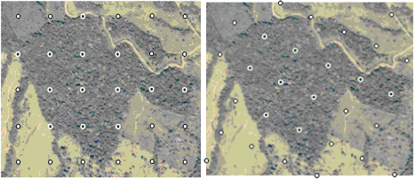
However, if this grid is superimposed randomly over the 1000 ha area of interest it is not guaranteed that always exactly the desired number of \(n=20\) sample points falls into the forest area. The number can be slightly higher or lower; that depends mainly on shape and fragmentation structure of the forest area, which is illustrated in Figure 2. What we have calculated here, actually, is not the sample size \(n\) but it is the expected value of the sample size \(E(n)\): on the average we have \(n\) samples in our area when repeating very often a random superimposition of the grid over the forest area.
| sorry: |
This section is still under construction! This article was last modified on 12/22/2010. If you have comments please use the Discussion page or contribute to the article! |

