Object-based classification (Tutorial)

Mean-shift segmentation of large size images

1. Step. We perform a mean shift filtering on the preprocessed input image 188_pca_cmask_8b.tif. (3 principal components of Landsat-8 multispectral bands (B1 - B7), pansharpened with band B8, rescaled to 8bit. Clouds and cloud shadows are masked). We extract homogeneous objects on the basis of a filtered image. Go to Processing-Toolbox --> Orfeo Toolbox (image analysis) --> Image Filtering --> Exact Large-Scale Mean-Shift segmentation, step 1 (Smoothing).
   1. • Set the 188_pca_cmask_8b layer as Input image.
      • The Range radius should be set to 30.
      • Leave all other configurations as they are and click Run. Have a look on the resulting filtered and spatial images.
2. Step. We convert the filtered image to one band image object. Go to Processing-Toolbox --> Orfeo Toolbox (image analysis) --> Segmentation --> Exact Large-Scale Mean-Shift segmentation, step 2.
   1. • The Filtered image is Filter output from step 1.
      • Leave the Spatial image as [not selected].
      • Range radius is set to 30.
      • Leave all other configurations as they are and click Run. The Output image is a labeled image where neighbor pixels whose range distance is below range radius will be grouped together into the same cluster.
3. Step. We adjust the image object size merging small regions with the module Processing-Orfeo Toolbox (image analysis) --> Segmentation-Exact --> Large-Scale Mean-Shift segmentation, step 3 (optional).
   1. • The Input image is the 188_pca_cmask_8b layer.
      • The Segmented image is Output image from step 2.
      • The Minimum Region size is set to 10.
      • Leave all other configurations as they are and click Run.
4. Step. We convert the image segments from raster to polygon vectors. Label ID, mean and standard deviation, number of the pixels in an image polygon are calculated and added as additional columns in the resulting shapefile.Processing-Orfeo Toolbox (image analysis) --> Segmentation-Exact Large-Scale Mean-Shift segmentation, step 4
   1. • The Input image is the 188_pca_cmask_8b layer.
      • Segmented image is Output image from step 3.
      • The name of Output GIS vector file is 1seg_188_pca_cmask_8b.shp
      • For the rest of parameters keep default values.Run.

Change Layer --> Properties Style --> Fill Style to No Brush and Colors --> Border to white. Overlay the vector file on top of the image 188_pca_cmask_8b.tif to evaluate the segmentation result.

Preparation of reference data

We join the Land use/cover (LUC) class attribute of manually digitized training areas with the image segments. Vector --> Data Management Tools --> Join Attributes by Location ....

1. 1. • The Target vector file is the Output GIS vector file of step 4.
      • Join vector layer is train_manual_poly.shp.
      • Output vector seg_188_pca_cmask_8b_train.shp.
      • For the rest of parameters keep default values.OK.

We need to rename the field names of the resulting output vector attribut table avoiding upper capitals and underslash using the Table Manager plugin.

Object-based classifcation using SVM algorithm

The vector based supervised classifcation modules in QGIS 2.12.3 are under development and still not working. Alternativly we may use the windows command line. Start --> All Programs --> OSGeo4W --> OSGeo4W Shell or double click on the file 'C:\OSGeo4W64\OSGeo4W.bat'. A windows command shell opens.

1. Type otbgui_ComputeOGRLayersFeturesStatistics
   1. • Name of the input vector is the file seg_188_pca_cmask_8b_train.shp.
      • XML file containing mean and variance of each feature is seg_188_pca_cmask_8b_train.shp.xml.
      • In the List of features to consider for statistics mark the columns meanB0, meanB1, meanB2.Execute.

Calcualte also an XML file for vector file seg_188_pca_cmask_8b.shp.

1. Type otbgui_TrainOGRLayersClassifier

1. Type OGRLayersClassifier

Info

For more detailed information on the SVM algorithm visit the library website

Alternative supervised classification with Support Vector Machine (SVM)

1. Start Monteverdi.
2. Open 188_pca_indices_pan_mean.tif and train_segments_7class.shp in Monteverdi via File --> Open dataset.
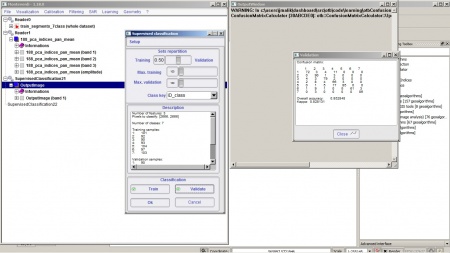
3. Go to Learning --> SVM classification (EXPERIMENTAL)
4. Load 188_pca_indices_pan_mean.tif as Input image and train_segments_7class.shp as Training/validation ROIs and press OK.
5. Specify the Class key as ID_class and click Train. A classification output is seen Monteverdi.
6. Click Validate to see classification accuracy and Calculate error matrix. See Figure G.

Supervised classification menu in Monteverdi with error matrix