Land Cover/Use Classification using the Semi-Automatic Classification Plugin for QGIS
(→Preparing raster data (Converting DN to reflectance)) |
(→Preparing raster data (Converting DN to reflectance)) |
||
| Line 15: | Line 15: | ||
[[File:Qgis_convert_boa_model.png|600px]] | [[File:Qgis_convert_boa_model.png|600px]] | ||
* Open the {{mitem|text=Processing --> Toolbox}} and {{mitem|text= Models --> Tools --> Add model from file}}. Load the previously downloaded model. | * Open the {{mitem|text=Processing --> Toolbox}} and {{mitem|text= Models --> Tools --> Add model from file}}. Load the previously downloaded model. | ||
| − | * The model should appear in the Models tab. | + | * The model should appear in the Models tab. |
| + | * Double click to open the model. | ||
* Assign the layers to the right band numbers. | * Assign the layers to the right band numbers. | ||
| − | |||
* Click {{button|text=OK}} | * Click {{button|text=OK}} | ||
Revision as of 18:00, 18 April 2018
Contents |
Working steps
Preparing raster data (Converting DN to reflectance)
- The Sentinel-2 products L1C and L2A are stored as digital numbers in data format unsigned integer 16bit. In this work step we scale the data to reflectance values with a new range from 0 to 1 and data type float 32bit.
- Load the single band raster file Subset_S2A_MSIL2A_20170619T_B2.tif and 9 other multipspectral bands (B3, B4, B5, B6, B7, B8, B11 and B12) of a Sentinel-2 scene.
- Open Raster --> Raster Calculator....
- Double click on a layer in the Raster bands list. The band should appear in the Raster calculator expression field.
- Complete the expression with the division operator // and 10000.
- Specify an Output layer path and name.
- Click OK
- Repeat these steps for all other multispectral bands.

- For this task you may also use a graphical processing toolbox model downloaded from here convert_L2A_reflectance.model (Right click, Save as ..).

- Open the Processing --> Toolbox and Models --> Tools --> Add model from file. Load the previously downloaded model.
- The model should appear in the Models tab.
- Double click to open the model.
- Assign the layers to the right band numbers.
- Click OK
- Follow Create stack to create a multiband raster file from the converted single bands and load into QGIS canvas.
Install and set up SCP plugin
- Click Plugins --> Manage and Install Plugins.
- Type in the search bar semi-Automatic Classification, click on the plugin name and then on Install plugin.

- Right-click on the Plugin Toolbar and make sure the following are checked SCP Dock, SCP Edit Toolbar, SCP Tools and SCP Working Toolbar.

Defining classification inputs in SCP-plugin
We need to define input image, training input and spectral signature files for SCP.
- Open the SCP Dock.
- Click SCP Dock --> SCP input --> Input image, use the button Refresh list
 and the drop-down menu-bar to select the multiband Merge file (i.e. from DN to Reflectance conversion) as input image.
- Click the button Band set
 to further define the input image.
- Next, click Quick wavelength settings and select Sentinel-2 from the list in order to automatically set the Center wavelength for each band and the Wavelength unit (NB. required for spectral signature assessment).
- In the RGB list
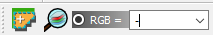 of the Working Toolbar, select 3-2-1 to display natural color composite. Also, type in 4-3-2 to display false color composite. While changing the color composite; also use the buttons cumulative_stretch
  and std_dev_stretch
  for better displaying the Input image (i.e. image stretching).
- We need to define training input file in order to collect ROIs and spectral signatures.
- Click SCP Dock --> SCP input --> Training input, use the button Create a new training input
 to create a training signature file with the extension .scp, click save.


Collection of ROIs and Spectral signatures
- Click on the button Add Vector Layer
 to Load the vector file Training_points_refactored.shp available in the course data and overlay it on the multiband Merge' layer.
- To display attribute labels for Training_points_refactored.shp, right-click to open Properties --> Labels. Select Show labels for this layer and Label with C_ID.
- ROIs can be created by drawing polygons using the button Create a ROI polygon
 or by an automatic region growing algorithm using the button Activate ROI pointer
  . The region growing algorithm can create more homogeneous ROIs (i.e. standard deviation of spectral signature values is low) than manually drawn ones; the manual creation of ROIs can be useful in order to account for the spectral variability of classes. We will use the automatic region growing algorithm.
- From SCP Dock --> Classification dock --> ROI creation, check the function Display NDVI.
- Next, click the button Activate ROI pointer , and notice that the cursor displays NDVI value which changes over the image pixels.
- Zoom-in to the points and click on a land cover/use pixel associated with the point attribute to create a ROI.
- On the Working Toolbar, increase the Dist parameter
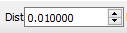 (e.g. from 0.010000 to 0.100000), and click the button Redo the roi at the same point
  to capture more of similar pixels.
- Still under SCP Dock --> Classification dock --> ROI creation, set MC_ID, C_ID, MC_info and C_info according to the point attribute (see attribute table), and click on the button Save temporary roi to training input
 to record spectral signature. Also set color for ROIs by double-clicking on Color from the ROI Signature list.
- Repeat step 6, 7 and 8, to record several land cover/use ROIs and spectral signatures for all points.


Assess Spectral Signatures
Premise: Different materials may have similar spectral characteristics. As such pixels could be misclassified due to inability of classification algorithms to correctly discriminate those spectral signatures. Thus it is important to review spectral signatures of training samples and repeatedly modify them until all class training sets achieve adequate spectral separability. This can be done by 1) displaying and assessing spectral plots and/or 2) calculating the spectral distances of signatures.
- Highlight spectral signatures in the ROI Signature list and click the button Add highlighted signatures to spectral signature plot
 to display signature plot.
- Disable/enable plot value range by checking/unchecking Plot value range.
- Observe differences in Pasture and Annual crops accross all wavelength ranges.
- Use the Automatic thresholds
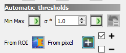 field to refine signature separability. It is also possible to refine the range within the plot. In the Plot Signature list, highlight a signature, click on the button Change value range interactively in the plot
  , click inside the plot to reduce or increase range. (NB. classes are well separated if there is no overlap in at least one band)
- For the highlighted signatures click the button Calculate spectral distances

- Click Signature details to unfold signature statistics for each wavelength range.
- Click Pectral distances to reveal spectral signature (dis)similarity metrics.
- To examine scatter plots for the highlighted signatures click the button Add highlighted items to scatter plot
 to display scatter plot.


Classification
Land cover/use classification
Create some classification previews to get an overview of how the process will perform. This also helps to improve on the spectral signatures of training input for better classification results.
- Click SCP Dock --> Classification dock --> Macroclasses to set the colours for each class.
- Then under SCP Dock --> Classification dock --> Classification algorithm, check Use MCID to use Macroclass IDs for classification. For the algorithm, select Maximum Likelihood and under Land Cover Signature Classification check the box next to LCS.
- On the Working Toolbar click the button
 to activate the classificatin preview pointer.
- Then click a point on the image to display a classification preview in the map. Use the button
 to zoom to the classification preview.
Classification can be performed after ROI creation and definition of spectral ranges.
- When satisfied with the preview and training input, check the box next to Algorithm under Land Cover Signature Classification.
- Open SCP Dock --> Classification dock --> Classification output and click the button
 to specify an output destination. Results will be displayed in QGIS canvas after the processing.
- Repeat with other algorithms to compare their performance.
Accuracy Assessment
Automatic multiple ROI creation
- Repeat the steps under Defining classification inputs in SCP-plugin to create a new training input file (this will be the validation dataset). Use Subset_S2A_MSIL2A_20170619T_B12_BOA.tif as input image
- Click SCP --> Tools --> Multiple ROI creation to set parameters for ROI creation using random points.
- Assuming we want to create 50 ROIs with a minimum distance of 500 map units from each other (to avoid overlaps), set Number of points to 50
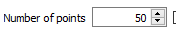 , min distance to 200
 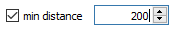 and keep the default ROI pixel size (i.e. Min 60 and Max 100)
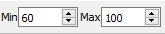 . Increase the Dist parameter to 0.5.
- Since we are not interested in ROI signatures, uncheck Calculate sig. , click Create points. and at the bottom right corner of the window and click the button to create multiple random ROIs.

Photo-interpretation of ROIs
The created ROIs will appear under ROI Signature list in the Creation Dock. Observe that all created ROIs have the same class information (i.e. MC_ID, MC_Info, C_ID and C_Info). Thus we need to assign the correct class to each ROI. This will be done by photo-interpretation with the aid of different color composites (to identifiy different features) and high resolution Google satellite scenes (for this purpose, install OpenLayers plugin).
- Click Web --> OpenLayers plugin --> Google Maps --> Google Satellite to open Google satellite scene in QGIS.
- In the Layer panel drag the Google satellite scene to overlay the Subset_S2A_MSIL2A_20170619T_B12_BOA.tif image.
- Double-click the first ROI under ROI Signature list to zoom in to the ROI.
- Open Properties --> Transparency and adjust the transparency of the Subset_S2A_MSIL2A_20170619T_B12_BOA.tif image to view the Google satellite scene and correctly assign ROI class information (i.e. MC_ID, MC_Info, C_ID and C_Info).
- Repeat steps 3 and 4 to assign the correct class information for each ROI.
NB: Class information for the validation data must be in conformity with the classification scheme in the training dataset.
Calculation of classification accuracy
This involves a comparison of the output land cover/use map from image classification with the independent reference/validation dataset. The result is an error matrix which allows for the computation of descriptive accuracy statistics for the overall classification exercise (i.e. overall accuracy) but also the accuracy of individual classes either as producer accuracy or user accuracy.
- Load the validation data (lab9_validation.shp) in QGIS.
- Open SCP --> Postprocessing --> Accuracy.
- Under Select classification to assess, use the button Refresh list and the drop-down menu-bar to select the output map from image classification.
- Under select the reference shapefile or raster, use the button Refresh list and the drop-down menu-bar to select the validation sample.
- Under Shapefile field, select C_ID and click the button to save the error raster and execute the process.

