Fixed area plots
| sorry: |
This section is still under construction! This article was last modified on 03/3/2011. If you have comments please use the Discussion page or contribute to the article! |
Contents |
General observations


Fixed area sample plots can have various different shapes including circular, square, rectangular and strip. As to which shape is chosen depends on practical and statistical issues. In terms of practical criteria it is mainly the cost which is of interest and which translates into criteria such as terrain conditions and expected frequency of border trees. Border trees cost time because it needs to be carefully checked whether they are in or not and that implies usually additional distance measurements which are not required for the other trees. From a practical point of view a circular plots is most rapidly installed wherever the visibility in the stand is good. In a tropical forest with dense understory, it is much easier to establish a strip plot where the field crew walks along the central line and measures all trees up to a defined distance to the right and to the left. A circular plot, however, has the lowest expected number of border trees, because, for a given area, the circle is the geometric shape that has the shortest perimeter.
From a practical point of view, coming back to the considerations on spatial autocorrelation, a long rectangular plot (strip plot) covers more different site conditions and is likely to capture more variability per plot. Thus, we may expect higher precision when using strip plots if we compare it with circular plots with the same plot area. In what refers to the plot size, for a given sampling intensity it is statistically more precise to establish many small plots than few large plots. However, with many small plots, again the cost will be much higher; the decision on plot size is again a compromise between practical (cost) criteria and statistical (precision). If there is some information on number of stems per hectare, one can calculate, as a rule of thumb, the plot area such that there are on average about 15-20 trees in a sample plot. Typical plot areas are 200 m², 500 m², 1000 m² - but anything is possible.
All trees that have the center of their base inside the plot area are sample trees and are being measured. If a tree is a border tree and it is not obvious whether it is in or out, a measurement must help with that decision. If the tree is exactly on the borderline, then one may count one tree and the next such tree not; but actually, when measuring distances with high accuracy, the case that a tree is exactly on the borderline should be very rare. It is only the center point of the tree base that defines whether a tree is in or out. If center point is in but the tree leans completely outside the plot, this is still an in-tree. If the center is not in the plot, but the entire tree leans into the plot, this tree is not observed.
The inclusion zone concept
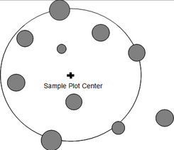
We introduced circular fixed area plots such that a sample point is selected and then all trees within a fixed distance (the plot radius r) are taken as sample trees (see Figure 46). While this plot perspective is intuitively clear and understandable, it does not allow to say anything about the per tree selection probability. This however, may be an important component of statistical information.
We may change the perspective from the plot perspective to the tree perspective. In that approach, we build a so-called inclusion zone around each tree. The inclusion zone is a measure for the selection probability of that particular tree: if a sample point falls into that inclusion zone, then this particular tree is selected. While this sounds maybe complicated, it is extremely helpful in understanding forest inventory sampling and also in deriving unbiased estimators for any plot design.
In the case of fixed area circular plots, the inclusion zone that is centered about each tree has the size and shape of the plot, that is circular. All trees, therefore, have the same selection probability. We now imagine the inclusion zones around all trees and select a sample point. Then, all those trees are selected as sample trees for which the sample point falls into their inclusion zone (Figure 47). Of course, at the end, exactly the same trees are selected as with the first approach (of laying out the sample plot), but in this second approach we take the selection probability explicitly into account.
The inclusion zone concept can be applied also to the other plot designs that are being presented in the rest of this chapter.
The plot expansion factor
Cluster plots
Nested sub-plots
Slope correction
Slope correction for line features
Effects of sloope correction
References
- ↑ 1.0 1.1 Kleinn, C. 2007. Lecture Notes for the Teaching Module Forest Inventory. Department of Forest Inventory and Remote Sensing. Faculty of Forest Science and Forest Ecology, Georg-August-Universität Göttingen. 164 S.