Study site
Several aerial missions equipped with airborne laser scanner (TopoSys Falcon II, Riegl LMS-Q560) and airborne digital camera (TopoSys line scanner, DLR HRSC-A) were flown in two forest districts in Northrhine-Westfalia in the years 2004-2007. The study sites Glindfeld (76km2) and Schmallenberg (280km2) are located in the low mountain range Sauerland in Northrhine-Westfalia, Germany. Main economically important tree species are spruce (Pices abies) and beech (Fagus sylvatica).
Displaying digital orthophotos (DOP)
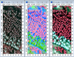
Figure A: Digital orthophotos (DOP), left: summer (RGB=432), right: winter (RGB=432), middle: first three components of PCA of 8 bands of DOP summer and winter.
- Start SAGA GIS: Start --> All Programs --> OSGeo4W --> SAGA GIS. If you do not find this link start the windows explorer, navigate to the folder C:\OSGeo4W\apps\saga. Copy the file
 saga_gui.exe and paste as a link on the desktop. Double click on the link symbol to start SAGA GIS.
- Find the file browser in the Data Source window in the the lower left of the SAGA Gui. Navigate to the path .\GBData\ALS where you saved the uncompressed tutorial data. Double click on the files so_abt49b1-Composite.sgrd, wi_abt49b1-Composite.sgrd and PCA-Composite.sgrd. Click on the Data Tab of the Workspace window to see the Data Tree. Double click on the first loaded layer to open a viewer window. Continue with the second and third layer and confirm always Map Selection New to open new cascaded viewer windows. Rearrange the viewers Window --> Tile vertically and link the viewers geometrically Map --> Synchronise Map Extent.
- Activate a layer by marking the layer in the Data tree. On the right side of the GUI is a window displaying the layer properties. Under Colors change the Type from Graduated color to RGB. Click Apply and repeat these steps for the other two layers (Fig. A). Place the cursor in one of the viewers. Zoom in with a left click and zoom out with a right click. Activate Pan
 to move the images. Describe the characteristics to distinguish the main tree species spruce and beech.
Displaying digital terrain model (DTM)
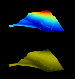
Figure B: Above: 3D perspective view of the DTM overlaid by stand boundaries (white). Below: red green anaglyph image of the DTM.
- In the Data Source window navigate to the path .\GBData\ALS, double click on the digital terrain model dtm_abt49b1.sgrd. The DTM in raster format was derived from the last pulse of ALS point data. Double click on the layer dtm_abt49b1 in the Data Tree to open a new viewer. In the properties of the layer dtm_49b1 on the right side of the Gui click the checkbox Show Cell Values on.
- Double click on the boundary of the stand compartment 49b1 boundary_abt49b1.shp in vector format. Double click on the Polygon layer boundary_abt49b1 in the Workspace. The stand polygon is displayed on top of the digital terrain model. On the right side of the GUI change the layer properties of boundary_abt49b1: Fill style: Transparent, Outline color white.
- Activate Zoom
 and left click several times into the viewer to see height above sea level as digital value of every raster cell.
- Zoom to full extent
 and then Show 3-D view
  . Select the grid system 1:469x 685y and Elevation: dtm_abt49b1. Change the display resolution to 1000. OK. Left click in the 3D viewer and hold to move the 3D perspective or press and hold the middle mouse button and move forward and backward to zoom in and out.
- Toggle the Anaglyph
 and put on stereo glasses with red for the left eye and cyan for the right eye to see the 3D effect (Fig. B).
Displaying airborne laserscanner (ALS) data
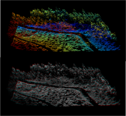
Figure C: Above: 3D perspective view of a ALS point cloud. Below: red cyan anaglyph image of a ALS point cloud.
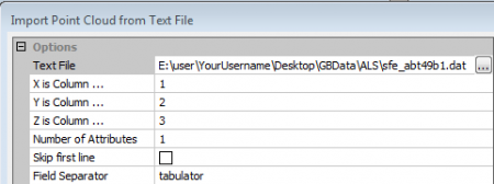
- Import ALS points into SAGA as tabulator separated text file with four columns: 1. Easting, 2. Northing, 3. Z and 4. Intensity. Modules --> File --> Shapes--> Import --> Import Point Clouds from Text File. Okay.
-
 Okay.
Okay. 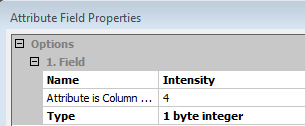 Okay.
Okay.
- Modules --> File --> Shapes --> Point Cloud --> Visualization --> Point Cloud Viewer. Specify Points: sfe_abt49b1.
- A Viewer opens. Click checkbox Central Projektion off and change the perpective view by holding the left click. Click checkbox Anaglyph on and put your red cyan stereo glasses on to see the 3D effect.
Generate a canopy height model (CHM)
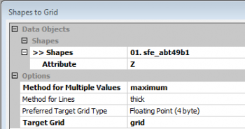
- Exract the top of the point cloud as first ALS reflectance and convert them to a rasterized digital surface model (DSM). Modules --> Grid --> Gridding --> Shapes to Grid.
-
 Okay.
Okay. 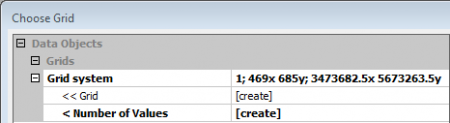 Okay.
Okay.
- Two new layers are created: sfe_abt49b1[Z] is the gridded DSM and sfe_abt49b1[Count] gives the point density per raster cell (here with area 1 m2). Mark the layer sfe_abt49b1[Count] in the Data tree. In the properties of the layer on the right side of the GUI click the checkbox Show Cell Values on.
- Have a look on the two created layers. Double click on the layer names in the Data Tree to open two new map views.
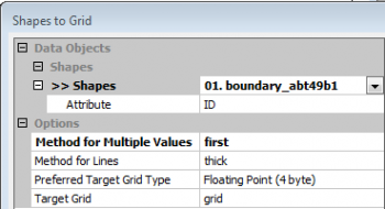
- Create a mask based on the stand polygon. Modules --> Grid --> Gridding --> Shapes to Grid.
 Okay.
Okay. 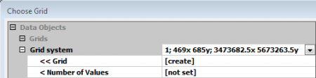 Okay.
Okay.
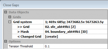
- We fill no-data areas of the DSM using the previous constructed mask of the stand polygon. Modules --> Grid --> Construction --> Close Gaps
-
 Okay.
Okay.
- Mark the new layer Changed grid in the Data Tree and change the Name to sfe_abt49b1_filled in the data properties on the right GUI side. Apply
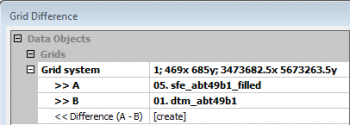
- We calculate the difference between the digital surface model and the digital terrain model. The result is a canopy height model (CHM) (Fig. D, E, F). Modules --> Grid --> Calculus --> Grid Difference.
-
 Okay.
Okay.
- Mark the new layer Difference (A-B) in the Data Tree and change the Name to canopy height model in the data properties on the right GUI side. Change the option for Colors and select on of the predefined Color Tables (e.g. red > grey > green) with Presets, Okay. Double click on the layer name in the Data Tree to open a new map view.
- Zoom to full extent and then Show 3-D view . Select the grid system 1:469x 685y and Elevation: canopy height model. Change the display resolution to 1000. OK. Left click in the 3D viewer and hold to move the 3D perspective or press and hold the middle mouse button and move forward and backward to zoom in and out.
- Toggle the Anaglyph and put on stereo glasses.
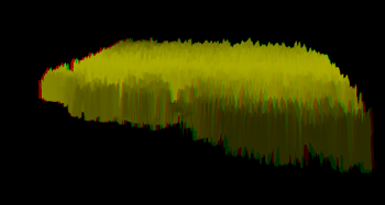 Figure D: Digital surface model (DSM) |
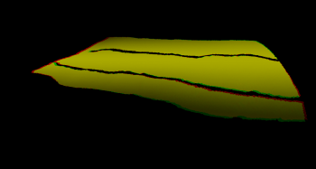 Figure E: Digital terain model (DTM) |
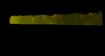 Figure F: Digital canopy height model (CHM = DSM - DTM) |
Individual tree detection
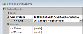
- Use a simple filter to extract minimum and maximum values in a local neighbourhood. Modules --> Shapes --> Grid --> Grid Values --> Local Minima and Maxima.
-
 Okay.
Okay.
- Two new shape point layers are created. Double click on the layer canopy height model[Local Maxima] in the Data Tree to open a new map view. In the properties of the layer on the right side change the Colors Type to Graduated Color and select Attribute: Z. Apply. Do you observe spatial trends of local maxima in the stand? Mark the point Layer canopy height model[Local Maxima] in the Data Tree, right click Histogram to display the height frequency distribution with a value range from -0,4 to 41.2.
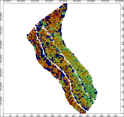 Figure A: Local maxima of the CHM |
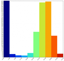 Figure B: Absolut frequencies of the CHM |
- Open the attribute table: mark the point layer canopy height model[Local Maxima] in the Data Tree, right click Attributes --> Show.
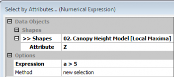
- As we are not interested in the understory we remove all points with Z < 5m. Modules --> Shapes --> Selection --> Select by Attribute... [Numerical Expression].
-
 Okay.
Okay.
- Modules --> Shapes --> Selection --> Copy Selection to New Shapes Layer creates a new layer canopy height model[Local Maxima][Selection] containing all points Z > 5m.
- Display the point layer canopy height model[Local Maxima][Selection] as an overlay of the PCA composite (s Fig. ) by double clicking in on the layer name Data Tree. and select the map viever of the PCA-Composite.
- Navigate to the path .\GBData\ALS. Double click on the file segments.shp to load a polygon shape layer with segments based on an automated tree detection based on a watershed algorithm. Double click on the layer inth Data treeand as Map Selection choose PCA-Composite. On the right side of the GUI change the layer properties Fill style: Transparent, Outline color: white (Fig. G).
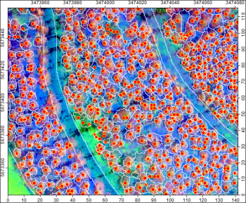
Figure G: PCA composite overlaid with local maxima and automatically generated tree crown segments (white).
Estimating top stand height
- Calculate the top stand height by using the mean of the 5% percent quantile from the upper end of the point layer canopy height model[Local Maxima][Selection]. Modules --> Shapes --> Points --> Point Filter.
- Find the result by marking the new created point layer Local Maxima][Selection][Filtered] in the Data Tree. In the data properties of the layer on the right side open the Description tab and find the top stand height as mean of the attribute Z.


