Exercise: Estimating top height of a forest stand by airborne laser scanning (ALS)
From AWF-Wiki
(Difference between revisions)
(→Displaying airborne laserscanner (ALS) data) |
(→Generate a canopy height model (CHM)) |
||
| Line 27: | Line 27: | ||
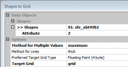
# Exract the top of the point cloud as first ALS reflectance and convert them to a rasterized digital surface model. {{mitem|text=Modules --> Grid --> Gridding --> Sapes to Grid}}. | # Exract the top of the point cloud as first ALS reflectance and convert them to a rasterized digital surface model. {{mitem|text=Modules --> Grid --> Gridding --> Sapes to Grid}}. | ||
| − | + | # [[Image:gridding1.png|250px]] {{button|text=Okay}}. [[Image:gridding2.png|250px]] {{button|text=Okay}}. | |
# Create a mask based on the stand polygon | # Create a mask based on the stand polygon | ||
# We calculate the difference between the digital suface model and the digital terrain model. The result is a canopy height model (CHM). | # We calculate the difference between the digital suface model and the digital terrain model. The result is a canopy height model (CHM). | ||
Revision as of 09:44, 18 July 2014
Contents |
Study site
Several aerial missions equipped with airborne laser scanner (TopoSys Falcon II, Riegl LMS-Q560) and airborne digital camera (TopoSys line scanner, DLR HRSC-A) were flown in two forest districts in Northrhine-Westfalia in the years 2004-2007. The study sites Glindfeld (76km2) and Schmallenberg (280km2) are located in the low mountain range Sauerland in Northrhine-Westfalia, Germany. Main economically important tree species are spruce (Pices abies) and beech (Fagus sylvatica).
Displaying digital orthophotos (DOP)

- Start SAGA GIS Start --> All Programs --> OSGeo4W --> SAGA GIS. If you do not find this link start the windows explorer, navigate to the folder C:\OSGeo4W\apps\saga. Copy the file
 saga_gui.exe and paste as a link on the desktop. Double click on the link symbol to start SAGA GIS.
- Find the file browser in the Data Source window in the the lower left of the SAGA Gui. Navigate to the path .\GBData\ALS where you saved the uncompressed tutorial data. Double click on the files so_abt49b1-Composite.sgrd, wi_abt49b1-Composite.sgrd and PCA-Composite.sgrd. Click on the Data Tab of the 'Workspace' window. Double click on the first loaded layer to open a viewer window. Continue with the second and third layer and confirm always Map Selection New to open new cascaded viewer windows. Rearrange the viewers Window --> Tile vertically and link the viewers geometrically Map --> Synchronise Map Extent.
- Activate a layer by marking the layer in the Workspace 'Data' tree. On the right side of the GUI is a window displaying the layer properties. Under Colors change the Type from Graduated color to RGB. Click Apply and repeat these steps for the other two layers (Fig. A). Place the cursor in one of the viewers. Zoom in with a left click and zoom out with a right click. Activate Pan
 to move the images. Describe the characteristics to distinguish the main tree species spruce and beech.
Displaying digital terrain model (DTM)

- In the Data Source window navigate to the path .\GBData\ALS, double click on the digital terrain model dtm_abt49b1.sgrd. The DTM in raster format was derived from the last pulse of ALS point data. Double click on the layer dtm_abt49b1 in the Workspace to open a new viewer. In the properties of the layer dtm_49b1 on the right side of the Gui click the checkbox Show Cell Values on.
- Double click on the boundary of the stand compartment 49b1 boundary_abt49b1.shp in vector format. Double click on the Polygon layer boundary_abt49b1 in the Workspace. The stand polygon is displayed on top of the digital terrain model. On the right side of the GUI change the layer properties of boundary_abt49b1: Fill style: Transparent, Outline color white. # Activate Zoom
 and left click several times into the viewer to see height above sea level as digital value of every raster cell.
- Zoom to full extent
 and then Show 3-D view
  . Select the grid system 1:469x 685y and Elevation: dtm_abt49b1. Change the display resolution to 1000. OK. Left click in the 3D viewer and hold to move the 3D perspective.
- Toggle the Anaglyph
 and put on stereo glasses with red for the left eye and green for the right eye to see the 3D effect. (Fig. B).
Displaying airborne laserscanner (ALS) data

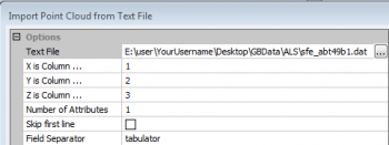
- Import ALS points into SAGA as tabulator separated text file with four columns: 1. Easting, 2. Northing, 3. Z and 4. Intensity. Modules --> File --> Shapes--> Import --> Import Point Clouds from Text File. Okay.
-
 Okay.
Okay. 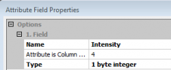 Okay.
Okay.
- Modules --> File --> Shapes --> Point Cloud --> Visualization --> Point Cloud Viewer. Specify Points: sfe_abt49b1.
- A Viewer opens. Click checkbox Central Projektion off and change the perpective view by holding the left click. Click checkbox Anaglyph on and put your red cyan stereo glasses on to see the 3D effect.


Generate a canopy height model (CHM)
- Exract the top of the point cloud as first ALS reflectance and convert them to a rasterized digital surface model. Modules --> Grid --> Gridding --> Sapes to Grid.
-
 Okay.
Okay. 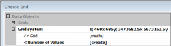 Okay.
Okay.
- Create a mask based on the stand polygon
- We calculate the difference between the digital suface model and the digital terrain model. The result is a canopy height model (CHM).
- Filling no-data areas.

